Notice: This Wiki is now read only and edits are no longer possible. Please see: https://gitlab.eclipse.org/eclipsefdn/helpdesk/-/wikis/Wiki-shutdown-plan for the plan.
Sample Projects available for Download
Contents
- 1 Sample Projects Available For Download
- 1.1 Importing a Shape File
- 1.2 Several Ebola Scenarios
- 1.3 Ebola Zoonotic Reservoir Model
- 1.4 Four Different Dengue Fever Scenarios
- 1.5 Avian Influenza (e.g. H7N9) Scenario
- 1.6 Malaria Population Replay Demonstration
- 1.7 Food borne disease
- 1.8 Migratory Birds Demonstration
- 1.9 Evacuation Demonstration
- 1.10 (Asia) Mosquito Density Model
- 1.11 Automated Experiment Example
- 1.12 Multi-Population Example
- 1.13 Multi-Population Pajek Graph Example
- 1.14 Square Lattice Example
- 1.15 Mexico/USA H1N1 Scenario
- 1.16 Global Earth Science Models
- 1.17 Global Geographic Models Only
- 1.18 Super-Continent Examples
- 1.19 Chicken Pox
Sample Projects Available For Download
The STEM home page contains several example projects users can import and run with STEM. These projects are intended to help users learn how scenarios are constructed and how to create their own. The examples demonstrate some, but not all, of the models available in STEM. Please see the documentation on Creating a STEM Scenario for more information on how scenarios are build as well as video tutorials. For users that want to add their own disease models (new disease and new code) please see Creating a new Disease Model Plug-in.
STEM is designed to allow collaboration and sharing of work by simply importing and exporting projects from your workspace. For information on how to import a project, please see: Importing and Exporting Projects
Sample Projects include:
- Ebola Scenarios
- Malaria population replay demonstration
- Food borne disease: Beef production from a cattle population
- Evacuation (Demonstration of Migration Edges)
- Chickenpox: The ChickenPox example scenario shows how to use the new aging (demographic) population model. The initial conditions in this example start the population far from equilibrium.
- Asia Mosquito Density Model Demonstrates how the earth science data can be used to generate seasonal mosquito density estimates in Asia. Requires the Global Geography Models and the Global Earth Science Models.
- Automated Experiment Example Demonstrates the automated experiment feature in STEM and how it is used to fit unknown EPI parameters to a reference incidence data set
- Global Earth Science Models for release 1.2.1 and later Continent-level models of Earth Science Data including elevation, rainfall, temperature, and vegetation coverage. OBSERVE: You need to access the STEM update site and install the "STEM Earth Science Data for 2010" plugin to use these models.
- Global Earth Science Models for STEM release 1.2.0 and earlier Continent-level models of Earth Science Data including elevation, rainfall, temperature, and vegetation coverage.
- Multi-Population Example Demonstrates a simplified multi-population disease model with anopheles mosquitoes and humans
- Pajek Import Example Demonstrates a simplified multi-population disease model where the entire graph is created using the new Pajek Import facility
- Square Lattice Example Demonstrates both population migration and disease spread on a Square Lattice
The Ebola scenarios require the latest STEM Integration build on or after Sept 26, 2014.
The malaria replay demonstration requires a build from Mar 16, 2012 or later
The evacuation intervention demo requires a build from July 15, 2011 or later
The Automated Experiment Example requires a STEM build from Sept 2, 2010 or later
The Multi-population Example requires a STEM build from Aug 31, 2010 or later
The Square Lattice demo described below requires STEM version dated July 1, 2010 or later
The SuperContinentExample project requires GlobalGeography to exist in the STEM workspace before it any of the examples can run
Some of the example projects you can download are very large as they contain continents or even groups of continents. Before you try to run any of these large scenarios you must make sure you allocate enough system memory for STEM. If you don't do this the application may hang or crash with a "Heap Space" error. To allocate enough memory in Windows, create a shortcut for launching STEM. You may place this anywhere (e.g., on your desktop or on the quicklaunch bar).
Right click on the shortcut. Select "Properties" You should see a field in the Properties Dialogue labeled Target: to the right in the text field you will see something like
C:\stem_builds\stem\STEM.exe -vmargs -Xms812M -Xmx812M
To launch STEM with more memory you must add "virtual machine arguments" to the target line. For example, Target:
C:\stem_builds\stem\STEM.exe -vmargs -Xms896M -Xmx896M
Should work for the demo projects available.
On MAC OS X, using the finder, navigate to where the STEM application is located, right click and select "Show Package Content". Navigate to Contents->MacOS and open the STEM.ini file in an editor. Change the -Xms and the -Xmx lines to increase the memory, e.g. -Xms896M -Xmx 896M or more depending on how much memory is available.
Importing a Shape File
You can download the .shp file example here. This example shows how to import geographic regions from a Shapefile and to create migration edges between these regions from a Pajek File. The files are located in the "Shapefile and Pajek" folder of the project. When importing the Shapefile the column "STUSPS" must be used for region IDs, since the Pajek File references these IDs. Please see the documentation on
Working with Graphs
- Composing a Graph
- Creating a Custom Graph (new) seasonal migration
- Visualizing and Editing Graphs with the STEM Graph Editor
- Importing a Graph from a Pajek File
- Importing a Graph from an Esri Shapefile
Several Ebola Scenarios
You can download the ebola models here. This archive contains multiple projects and multiple scenarios for Ebola. The archive also contains the Ebola model itself which can be opened and edited with the STEM model generator. Click on the page Ebola How To for more information on how to install and run the models. For more information on the model itself please see the page Ebola Models
Ebola Zoonotic Reservoir Model
This Downloadable Scenario contains an archive EbolaZoonoticReIntroduction. The archive contains two sub-folders.
 EbolaSingleNode
and
 org.eclipse.stem.ebola2
Both of these folders should be extracted and placed directly in your stem workspace. Do NOT put them in a subfolder inside the workspace
org.eclipse.stem.ebola2 contains the metamodel with extensions to the ebola model to support modeling of reintroduction
of ebola from a zoonotic reservoir.
EbolaSingleNode is a standards STEM project with a single node scenario. The disease decorator within instantiates the custom org.eclipse.stem.ebola2 ebola model
See: STEM_Model_Creator for information on metamodels and the model generator
Four Different Dengue Fever Scenarios
This folder contains four different scenarios (in four project folders) of dengue disease transmission in order to show behaviors observed from three dengue models with different levels of complexity. Details of each model can be obtained in our JTB paper (Hu. et al, “The effect of antibody-dependent enhancement, cross immunity, and vector population on the dynamics of dengue fever”, 2013.) and wiki page on the Dengue Fever Disease Models. Additional information on these downloadable dengue scenarios may be found on the page Downloadable Dengue Scenarios and in the readme.pdf file contained in the download.
To run the scenarios, first download the archive DengueScenarios.zip then extract the archive. You will see four subfolders, DengueVerySimpleModelTest, DengueHostVectorModelDemo, and DengueInAustralia. There are four separate STEM projects you can run. The DengueHostVectorModelDemo contains two scenarios within.
To import the project, run stem and then:
>File>Import>Existing Projects Into Workspace
>Select 'Next'
Make sure the radio button 'Select root directory' is checked (and no the archive button).
Then Browse or navigate to the parent folder 'Dengue Scenarios'.
>Select 'Next'
You can then import all three scenarios.
Avian Influenza (e.g. H7N9) Scenario
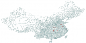
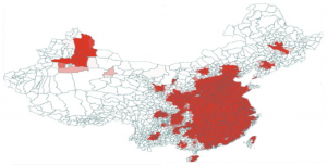
In response to 2013 China H7N9 outbreak in China we created an Avian Influenza Model and the following downloadable scenario. This scenario shows the possible disease propagation on the map of China seeded in Shanghai, China. The model includes air travel. By tuning the disease parameters, one can study sensitivity of spatial and temporal disease diffusion. In particular the scenario shows how the epidemic would change if direct human-to-human transmission were to occur (in the 2013 epidemic the only human cases came from poultry-to-human transmission.
Stochastic H7N9 simulation with poultry-poultry and poultry-human transmission. Watch on YouTube Poultry-Human Transmission
Stochastic H7N9 simulation including poultry-poultry, poultry-human, and human-human transmission (with air travel). Watch on YouTube Human-Human Transmission
Malaria Population Replay Demonstration
In this demo, we are reading in a time series of Anopheles population data for 71 regions in Thailand and use it to drive a model of Malaria transmission. Seasonal counts of anopheles mosquitos are recorded, as well as counts of births and deaths. You'll notice that the data being read in was recorded earlier using the CSV logger in STEM and that the ExternalDataSourcePopulationModel is configured to read data from the folder containing the run parameter file as well as an XMI serialized version of the decorator generating the data. This gives us the flexibility to replay population data for more exotic kinds with non-tranditional labels. The same rule applies for disease model data read by an ExternalDataSourceDiseaseModel.
If your data files were not generated by STEM, you can still use an ExternalDataSourcePopulationModel and point it directly to the folder containing CSV data files. The folder must contain a file Count_x.csv (where x is the administrative level of the regions recorded in the file, e.g. 2) and use the same format as STEM log files. The folder can optionally contain the files 'Births_x.csv' and 'Deaths_x.csv' to indicate the number of births and deaths of the population in each time step. This information is feed into any disease model using the external data source population model. If births and deaths data is not available, it is assumed that any increase in population is due to births only (zero deaths) and any decrease is due to deaths only (no births). Similarly, if there is a mismatch in the reported birth and deaths compared to the reported total count, the birth and deaths are adjusted to make up for the difference. This can happen for instance if you recorded data from a STEM simulation that had population migration as part of the model.
Food borne disease
African Swine Fever
new! This downloadable scenario contains both spacial and non-spacial African Swine Fever models. Please visit the African Swine Fever for details.
1. Beef Production
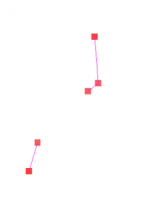
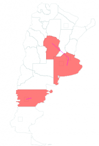
The BeefArgentina scenario is a model of beef production and consumption in Argentina using the new SlaughterHouse and FoodConsumer classes. The graph containing the cattle population, cattle transportation and slaughterhouses was created with the Pajek importer. The edges for beef transportation from this graph to the Argentina graph were created with the Graph Editor. Disease transmission from cattle to beef to human is also modeled.
Three of the nodes in the Pajek imported graph shown in the left image contain cattle populations. Cattle are born there and transported to the two nodes that contain slaughterhouses. In these nodes cattle is transformed to beef by using the SlaughterHouse class. The SlaughterHouse also models disease transmission in the transformation process (for example: 90% of infectious cattle transform to infectious beef and 10% to non-infectious beef). Beef is transported from the SlaughterHouse nodes to certain regions in Argentina as shown in the right image. In the Argentina graph beef consumption is modeled using the FoodConsumer class. This class also models disease transmission from beef to humans by consumption.
The downloadable archive contains the Pajek file for the graph.
2. A scenario for modelling the transmission of Salmonella to pigs, pork and humans
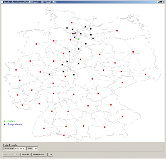
Food poisoning is caused in many cases by Salmonella. In this model the spread of Salmonella from farm to fork is demonstrated for the production and consumption of pork in Germany based on findings from the scientific literature. It shows the spread of Salmonella among pigs in a barn, the contamination of pork by infected carcasses in slaughterhouses, and the infection of humans with contaminated pork.
Salmonellosis in pigs
The infection of pigs with Salmonella is modelled with a compartment model (SIR). Soumpasis and Butler (2009) calculated that the transmission parameter β equals 0.165. They reviewed the literature and found that infected pigs stop shedding Salmonella after 16 days (1/γ = 16 -> γ = 0.0625) and that pigs become susceptible to salmonellosis after 42 days (1/𝛼 = 42 days -> 𝛼 = 0.0238).
The scenario is set on a farm for pig fattening with a population of 400 pigs (called “PigFattening”) in one barn (300 m2). Thus, there are 0.75 m2 per pig. 1 % of the population (= 4 pigs) was assumed to be infected with Salmonella. A reason for the appearance of Salmonella in pigs on a farm could be that the farmer buys several pigs of which four are already infected, for example. Pigs were fattened for 120 days. The model calculated 16 % of the pigs to be infected with salmonellosis. According to Methner et al. (2011), 13.8 % of 1830 fattening pigs were infected with Salmonella, meaning that the result of the model parameters published by Soumpasis and Butler (2009) is alright for an approximation.
Transport of pigs to slaughterhouses and contamination of pork with Salmonella
Pigs were transported to one slaughterhouse in Hamburg and Braunschweig each (60 % and 40 % of the population, respectively). Transport was assumed to take one day. The possibility of infection during transport and lairage was not calculated. There are several publications with models for the transmission of pathogens during lairage and slaughter. These are usually complex models with compartments different from the standard SIR compartment models. Van der Gaag et al. (2004), for example, use an enhanced compartment model, in which a carrier state and an additional state of infection (S-I-I-C) are proposed for carcasses. This model is currently not yet implemented in STEM and this is why only the prevalence of Salmonella in pork was used. In 2009, 2.5 % of the pork samples in Germany were Salmonella positive (BfR, 2011). Thus, the transmission rate was calculated using the published 14 % of infected pigs (Methner et al., 2011) and 2.5 % contaminated pork. This takes into account that roughly 70 % of the contamination of pork is a result of the pig being infected and 30 % is due to cross-contamination of pork from non-infected pigs with contaminated surfaces or machines (Berends et al., 1997). The contamination rates can be calculated from these values:
| |
S |
I |
| S |
0.991 |
0.009 |
| I |
0.875 |
0.125 |
| R |
0.991 |
0.009 |
The transformation of pig to pork was set to 1:200, meaning that a fattened pig – weighing about 100 kg on average – was processed to 200 pieces of pork (500 g each). Pork is transported to several shops in northern and central Germany and is sold instantly at 100 %. An increase of the Salmonella concentration due to inappropriate cooling and the possibility that not all units of pork might be sold were not taken into account.
Infection of humans with salmonellosis from pork and human-to-human transmission
According to a study from The Netherlands, 95 % of all human salmonellosis cases are foodborne and only 5 % from human-to-human transmission (Berends et al., 1998). In 2009, 31,400 human salmonellosis cases were reported in Germany (RKI, 2012). In general, about 20 % of salmonellosis cases can be attributed to the consumption of pork (Steinbach and Kroell, 1999) (here: 6280 cases). However, this model computes the spread of foodborne Salmonella for only a part of Germany with much smaller numbers of pigs for only a part of the year. This is why the number of infected humans is much smaller in the described model.
How the Salmonella scenario was built in STEM
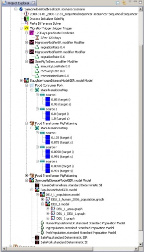
We started with a new model (PopulationModelGER.model) and dragged a population model for the country of interest into the new model (here: DEU_1_population.model). We defined the so called “population models” (symbol: man standing) for each population (human, pig, pork) and dragged them into the new model, by right clicking on the “PopulationModelGER.model” and then clicking on “Display canonical graph”. A window opened showing the chosen country with nodes containing the area and the human population.
By right clicking we added a node, named it, and defined its size. Next we right clicked this new node and added population labels for each population we wanted to assign to this node. The pig farm needed a label for the pig population (called “PigFattening”) and we added new nodes for slaughterhouses. (Because pigs are processed to pork, these nodes need labels for both pig and pork populations.) To define the transport of pigs from the farm to a slaughterhouse, we highlighted both nodes (Ctrl + left click), chose “Add migration edge,” and named the population to be transported (here: “PigFattening”) and how many pigs would move.
While the “rate” is a percentage of the whole population in the farm, checking the box “Use Absolute Value” enabled us to specify how many individual pigs should move each time interval. “Period” defines this time interval (default is 86400000 ms = 1 day). Pork migrates from slaughterhouses to retail and from there to the counties. This way all the retail facilities were connected to slaughterhouses on one side and to county nodes on the other side. We added the “Pork” population to retail and county nodes, clicked “Save Graph,” and “Quit.” Moving to Project Explorer, we defined new diseases for the transmission of salmonellosis between pigs and from pig to pork. Here we entered the data found in the literature, dragged the diseases into our model (here: PopulationModelGER.model), and defined a new model (SalmonellaDiseaseModelGER.model) that contained the PopulationModelGER.model and a new disease for human salmonellosis (HumanSalmonellosis.standard Deterministic SI).
Next we defined a last model for the transmission of Salmonella from pig to pork (SlaughterhouseDiseaseModelGER.model). This contained the SalmonellaDiseaseModelGER.model and two other items: the food consumer and the food transformer. We created both by clicking the plant symbol “Create a new Population Transformer”and picking the population transformer “Slaughter House” to transform pig to pork. When we entered the correct name of the source and target population, the diseases were chosen automatically (if there is only one disease like in this description). We chose which node should represent the slaughterhouse by picking the target location, choosing “select within project,” and highlighting a node (here: SlaughterHH). We used the “Food Yield Multiplier” to define how many units of pork are processed from one pig and “Disease Mapping” to configure the proportion of pork that would be either free of or contaminated with Salmonella. After we finished this population transformer, we defined another one for the second slaughterhouse (here: SlaughterBR).
We added another population transformer called “Food Consumer” to our scenario to model the consumption of pork by humans. In this case we did not pick a target location because we assumed the whole human population should be able to eat pork.
We placed the two food transformers and the food consumer in the model “SlaughterhouseDiseaseModelGER.model” and dragged the latter into a new scenario. As always, when we built the scenario, we included a sequencer and defined a disease initializer. In order to start the transmission of Salmonella between pigs, we right clicked on the disease “SalmPig.standard Deterministic SIR” and clicked “Create new Initializer.” We then chose the pig population (“PigFattening”) and defined the number or fraction of pigs being infected. The location was the pig farm.
In our scenario, the pigs fattened for 120 days with no migration of pigs from the pig farm to the slaughterhouses until day 120. To reflect this, we used a migration trigger with a predicate (120 days) and migration modifiers (definition of the proportion of pigs migrating to either slaughterhouse).
That’s what we did to build our scenario. Now you can start the simulation.
References
Berends BR, Van Knapen F, Snijders JM, Mossel DA. Identification and quantification of risk factors regarding Salmonella spp. on pork carcasses. Int J Food Microbiol. 1997 May 20; 36(2-3):199-206. PubMed PMID: 9217109.
Berends BR, Van Knapen F, Mossel DA, Burt SA, Snijders JM. Impact on human health of Salmonella spp. on pork in The Netherlands and the anticipated effects of some currently proposed control strategies. Int J Food Microbiol. 1998 Nov 10; 44(3):219-29. PubMed PMID: 9851601.
BfR (Federal Institute for Risk Assessment). BfR Wissenschaft – Erreger von Zoonosen in Deutschland im Jahr 2009. Hartung, M. and Kaesbohrer, A. (eds.); 2011
Methner U, Rammler N, Fehlhaber K, Rösler U. Salmonella status of pigs at slaughter--bacteriological and serological analysis. Int J Food Microbiol. 2011 Nov 15; 151(1):15-20. Epub 2011 Aug 3. PubMed PMID: 21872961.
RKI (Robert Koch-Institut), SurvStat, http://www3.rki.de/SurvStat, accessed on April 11th 2012
Soumpasis I, Butler F. Development and application of a stochastic epidemic model for the transmission of Salmonella Typhimurium at the farm level of the pork production chain. Risk Anal. 2009 Nov 29 (11):1521-33. Epub 2009 Jul 31. PubMed PMID: 19659452
Steinbach G, Kroell U. [Salmonella infections in swine herds--epidemiology and importance for human diseases]. Dtsch Tierarztl Wochenschr. 1999 Jul; 106 (7):282-8. German. PubMed PMID: 10481371.
Van der Gaag, M.A., Vos, F., Saatkamp, H.W., van Boven, M., van Beek, P., Huirne, R.B.M. A state-transition simulation model for the spread of Salmonella in the pork supply chain. European Journal of Operational Research 2004 Aug 1; 156 (3): 782-798, ISSN 0377-2217, 10.1016/S0377-2217(03)00141-3; (http://www.sciencedirect.com/science/article/pii/S0377221703001413).
Migratory Birds Demonstration
The Migratory Birds project demonstrates how the Seasonal Migration Edge Graph Generator can be used together with a Seasonal Migratory Population Model to create models where animals migrate seasonally between regions.
known issue: If you edit this model and if you replace the finite difference solver with a Stochastic Solver the birds will not migrate.
This occurs because the stochastic solver requires that you have a disease model in your scenario (and this example scenario only includes the population).
The  issue only applies to use of a stochastic solver. The simple fix is to create a disease and add it to your model.
You can keep a transmission rate of 0.0. Then it will run fine.
Remember to set the target population or your disease to 'birds' matching the name of the population.
Evacuation Demonstration
The evacuation demonstration project aims to demonstrate how interventions can be used in STEM to control an outbreak. In this simple example, we have two regions (Square 0 and Square 1). The regions are connected by symmetrical migration edges moving 5 % of the population from region 0 to region 1, and 5 % of the population from region 1 to 0 in each time step. Hence the total population count is preserved in each region.
Region 1 has a hospital. The hospital is represented by a intervention label inside the HospitalGraph.graph file. You'll see that the hospital has the capacity to vaccinate 50 people per time step (daily).
In the scenario "NoEvacuationsScenario", an outbreak occurs in region 0 and no intervention takes place. Via migration the disease also spreads to region 1.
In "EvacuationScenario", after more than 5 cases per day occurs in region 0, an intervention policy is triggered. The policy does the following:
1. It cuts off any migration of people from region 1 to region 0.
2. It increases the migration of people from region 0 to region 1 (where the hospital is).
3. It increases the vaccination capacity of the hospital from 50 per day to 100 per day.
Once the number of cases in region 0 drops below 5 per day again, migration and vaccination are set back to their original settings
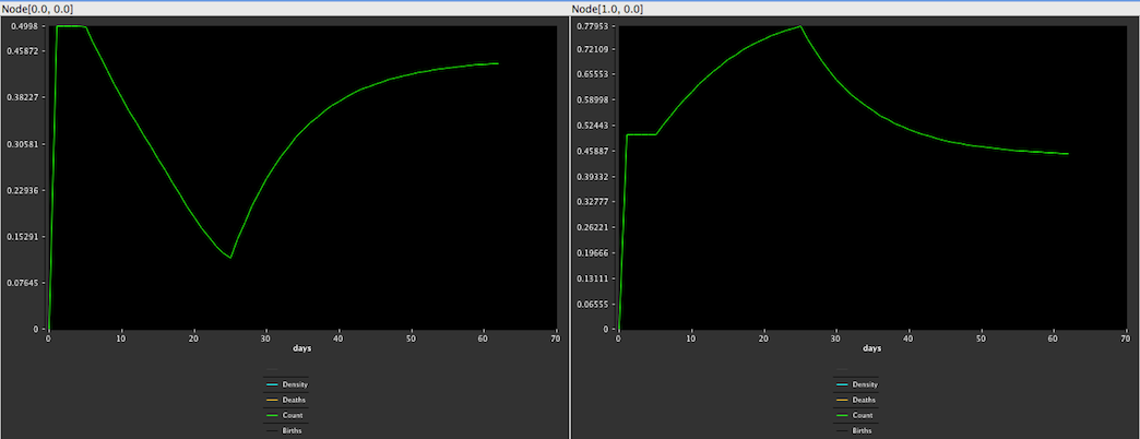
In the figure below, you'll see that the policy triggers around time step 6 and the population numbers starts dropping in region 0 due to evacuation. Correspondingly, the population increases in region 1. When the outbreak is under control at around time step 25, the migration is balanced out and the population numbers converges back towards the original values.
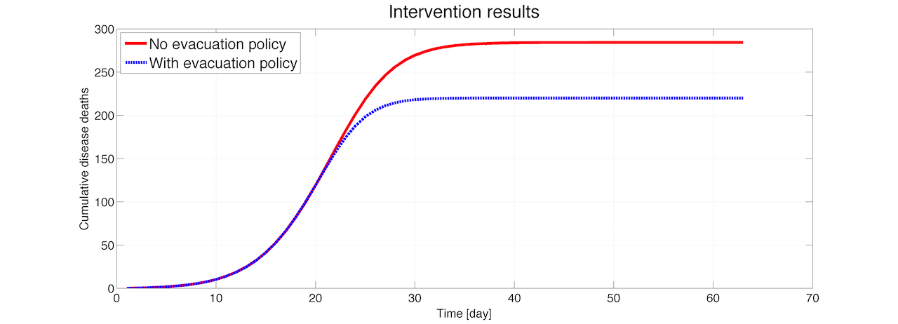
If we look at the cumulative disease deaths occurring in both scenarios, the figure below indicates that by evacuating and increasing vaccination capacity, a total of about 65 lives are saved.
(Asia) Mosquito Density Model
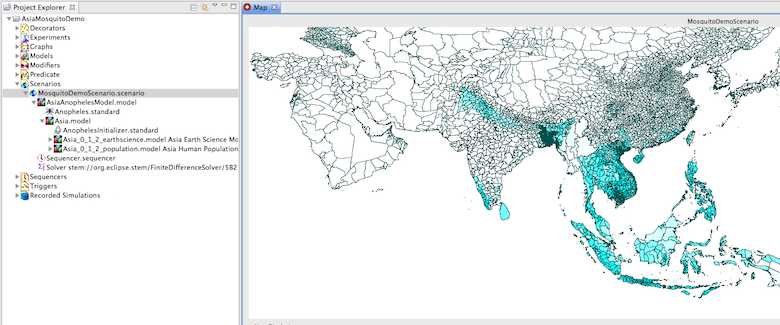
This downloadable scenario demonstrates how the earth science data can be used to generate seasonal mosquito density estimates in Asia. Before you try to run this scenario you much also install the STEM Earth Science Data Feature for the year 2010 (the year used in this example). The scenario (configured for Asia) also requires the Global Geography Models and the Global Earth Science Models available on the STEM Downloads page. You can easily reconfigure this scenario for the entire globe or for other selected regions. The screenshot below shows the Asia Mosquito Model running as downloaded. On the right hand side in the Project Explorer the scenario is expanded to show how it is constructed. The model contains the prebuild Global Geography Model (Human) for Asia along with its polygons, nodes, and edges, as well as the corresponding Asia earth science model (this in turn contains rainfall, temperature, vegetation, and elevation data for the same regions of Asia). These, together with an Anopheles Initializer, are contained in a parent model simply called Asia. The parent model along with the STEM population model for Anopheles are placed in the parent scenario. Users may easily modify this to study other regions. In the future the Anopheles model will be used as part of a complete vector disease model for Malaria and other conditions.
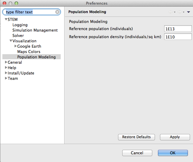
Notice: You probably need to change the reference population and reference population density in the STEM preferences to ensure the map colors are not saturated. When STEM determines the intensity of the color used to fill regions on the map, it takes the actual count (in case the number of Anopheles mosquitos) and divides by the reference population. The number between 0 and 1 (if it's larger than 1 it's set to 1) determines the intensity of the color. See screenshot below for numbers that are reasonable for this particular scenario:
Automated Experiment Example
In this example, we have been given historical incidence data for a disease with unknown epi parameters and we want to try and determine what those parameters are. All we know is that the first cases showed up in Stockholm. If you import the demo project into your workspace, the reference incidence data is located under the "Recorded Simulations/Reference" folder in the Incidence_1.csv file (the other files in the folders are not used in this example).
We decide to try and fit an SIR model to the incidence data, and we would like to determine three unknown parameters:
1. What was the transmission rate of the outbreak?
2. How long were infected individuals shedding viruses (i.e. recovery rate)?
Given these two parameters it's possible to determine the reproductive number of the disease, an important epi parameter.
We also have one more unknown we would like to estimate
3. What was the initial background immunity to the disease.
Next, open the "Experiments" folder in the project explorer and double click "AutomatedExperiment.autmaticexperiment" it to bring up its editor. Select the top node in the editor and look at its properties in the properties view.
Automatic Experiment Editor
You will notice that the automatic experiment will run a scenario called "AutomatedExperiment.scenario". This is a basic SIR scenario where with a few initial cases of the disease occuring in Stockholm, as well as an inoculator to initialize the background herd immunity. You will also see that the algorithm being used to fit parameters to the reference is called "Nelder-Mead", and that an error function called "Simple error function" is used. Nelder-Mead is a well-known numerical model optimization algorithm, and the "Simple error function" calculates a normalized root mean square error between the incidence reported in the reference and the incidence calculated by the model simulation. The incidence is aggregated over all locations that are common between the model and the reference.
You'll also see that the maximum number of iterations is 1000. This means that at most 1000 simulations are run before either the algorithm stops or it restarts itself using the optimal set of parameter values found so far. If "Reinit" is false, the algorithm stops after either a solution having an error tolerance smaller than the one specified (1E-6) is found, or the maximum number of iterations is reached. If "Reinit" is true, the algorithm restarts itself again and stops only when the the solution converges towards the same minimum twice.
If you expand the top node "AutomatedExperiment.autmaticexperiment" in the editor you'll see that the automated experiment has 3 parameters it attempts to fit:
1. transmissionRate. The initial guess is 0.8 and the algorithm will use a step size of 0.2 when walking the parameter space for this parameter. Also, the maximum and minimim values for this parameter is 0.001 and 10. You can modify any of these values in the properties view.
2. recoveryRate. The initial guess is 0.2, step is 0.3 and the parameter value is between [0.001, 2.0]
3. inoculatedPercentage. The initial guess is 20, the step is 30 and the parameter is between [0,100]
All three parameters also reference the model the parameter belong to, in this case the first two reference the disease model and the last reference the inoculator.
To start running the automated experiment, right click on the "AutomatedExperiment.autmaticexperiment" file in the project explorer and select Run. STEM will automatically switch to the Automated Experiment perspective and the Automated Experiment view.
You'll see a view with tab options on top ("Error Convergence", "Incidence vs Time" etc.). Select "Current Values". You'll be shown a scrolling list of parameter values and to the right you'll see the calculated normalized root mean square error for that set of parameters.
The history of parameter values and the associated error is shown in the Current Values view.
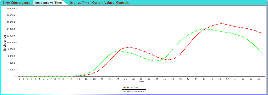
The "Error Convergence" shows a graph of the calculated error for each simulation and you'll notice how the error gets smaller and smaller. "Incidence vs Time" shows the latest incidence calculated by the current set of parameters compared to the reference incidence. Click the link below to see an animation demonstrating how the incidence is converging towards the reference.
The current calculated incidence versus the reference incidence Click here to see animation
"Error vs Time" shows the difference in incidence between the reference and the current model, compared to the difference in the best fit found so far. Finally, you can stop and restart an automated experiment using the "Contols" tab. When it looks like the algorithm has converged and the error is not changing much it is often useful to stop the experiment and restart it manually using the current optimal set of parameter values found. You can also specify any other parameter values on the Controls page and restart the experiment from those.
If you let the algorithm run until it completes (after about 340 simulations), it ends up with the following estimates for the parameters:
- transmissionRate: 1.199874
- recoveryRate: 0.30012
- inoculatedPercentage: 34.9852
You've probably already guessed it, but the reference data in this case was actually generated using a model with known parameter values. The values were 1.2 for transmission rate, 0.3 for recovery rate and the inoculated percentage was 35% (you can try plugging these values into the automated experiment, the error returned should be 0). You can force the algorithm to search for an even better fit by lowering the Tolerance parameter in the automated experiment (the tradeoff being that it takes longer to finish).
Each combination of parameter value tried and the resulting error is stored in a file called resultLog.csv in a folder AutoExpTempDir in the STEM workspace.
Multi-Population Example
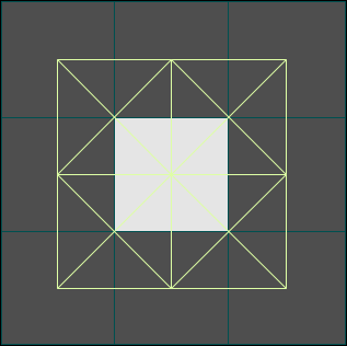
Figure 1a-b. Square lattice world where the anopheles and human population is evenly distributed on each lattice square (a), and where there is a human village located in the center square (b). The edges are the common borders where both anopheles mosquitos and humans are mixing.
The Multi-Population example contains two scenarios of very much simplified Malaria models spreading across a 3x3 square lattice world. In the first example (Figure 1a), each node contains the same number of humans (50) and the same number of anopheles mosquitos (10,000). In the second example (Figure 1b), there is a village in the center square lattice containing 1,000 humans.
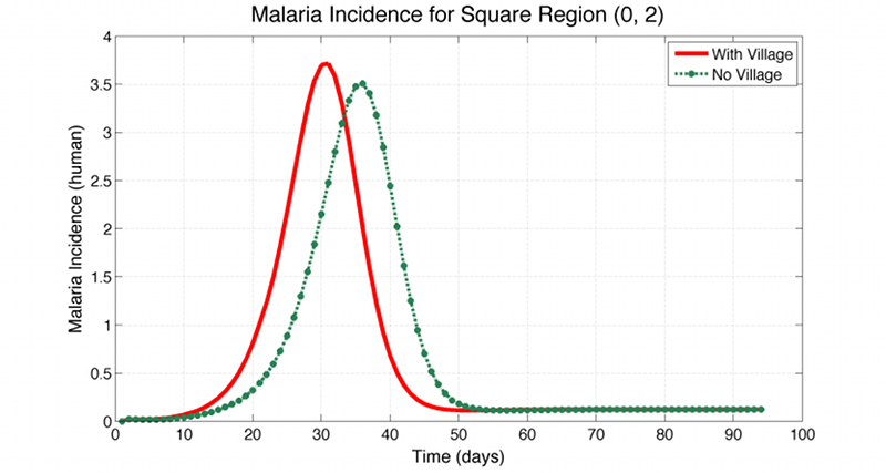
The disease is only spreading from infected humans to susceptible mosquitos or from infected mosquitos to susceptible humans, and it starts off by infecting 5 anopheles mosquitos in the upper left square. No infections transmit directly from human to human or mosquito to mosquito. The example also contains the log files from both scenarios, and a comparison between the incidence in the lower right square for both scenarios is shown in Figure 1c below. As can be seen, with the village in place, the incidence peaks about a week earlier for the lower right square. It should be noted, that in this simple sample model the mixing between anopheles members in two neighbouring nodes is at the same rate as the mixing between the human members of the very same nodes. In a real world example one would have to specify these rates seperately.
Figure 1c. Comparison of the daily incidence for both scenarios available in the Multi-Population example. In the scenario having a village in the center square, the incidence in the lower right square peaks about a week earlier than without the village.
Multi-Population Pajek Graph Example
Please find documentation for this downloadable scenario on the wiki page Importing a Pajek Graph.
Square Lattice Example
Figure 2. Square Lattice Example
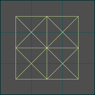
The Square Lattice Example shows how a square lattice, migration edges, and initial population gradient can be used to model the interaction between an infected and uninfected population. It also demonstrates the hierarchy required to set up a SquareLatticeScenario.scenario: disease models must contain population models, and population models must contain initialized graphs, etc.
As illustrated in the figures that follow, the Square Lattice Example shows how to use migration edges to create two population gradients that cause a population to spread out over space and time. Only one of two populations is initially infected with a disease so you can see both the spread of disease within the original population as well as the eventual transmission from the infected population to the susceptible group when they meet. To accomplish this, the example uses both a standard population model and a Population Initializer (see Figure 1 below and the Tutorial on Using Structured Populations). The population initializer places an initial number of individuals at two separate locations at time zero. Migration edges exist (with equal migration rates) in both directions between all sites but, because there is a population gradient, the population spreads out or diffuses across the lattice.
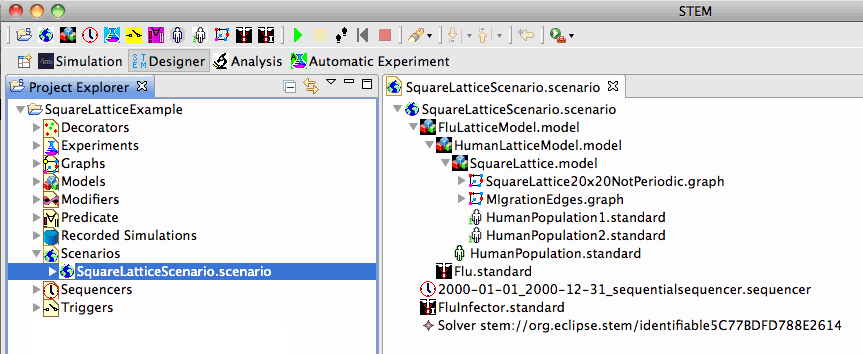
Note that the components that appear when you click on SquareLatticeScenario.scenario (Figure 2, right) are hierarchical. The two population initializers are placed within the innermost option, HumanPopulation1.standard. The standard population object (HumanPopulation.standard) depends on the existence of the initialized graph and, therefore, is placed in the outer HumanPopulationModel. Both of these submodels are components or bundles that can be reused across many scenarios. Finally, the disease itself (Flu.standard) is a human disease that depends on a contained human model so it is placed in the outermost model of the hierarchy (FluLatticeModel). This too is a reusable component.
The Infector for the disease (FluInfector.standard) depends on a model of what is already known about the disease. An infector changes the state of a model by moving individuals from the susceptible state to the infectious state (given the presence of the indicated disease). As such, an infector is really part of the scenario - the topmost level in the hierarchy that contains ALL models.
In the figures below, you can see the initial population spread by migration edges. In the same simulation at runtime you can select the disease as the property to display and watch the disease spread.
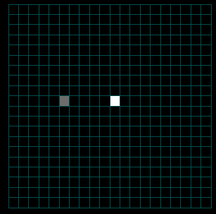
Figures 3a-c. Spread of the Human Population by Migration Edges
The figures above show the spread of the population itself by migration edges. The population is seeded in the center (10x10) and in a node just left of center. The center population is much larger than the smaller seed to the left (the intensity is saturated). Only the population to the left is infected initially. Open the infector and the population initializer in the property editor to see the initial values. As the infected population on the left spreads, it eventually makes contact with and infects the main population spreading from the center.
Figures 4a-c. Spread of the Disease
The figures above show the same simulation but display the fraction of people infected as a function of time. Note that the intensity does not reflect the NUMBER of infections (only the fraction). When the infected population on the left reaches the much larger fully susceptible (but not yet infected) population spreading from the right, the intensity actually goes down as the fraction of people infected drops (initially) at the point of contact (see the middle image above). Eventually (right) the main population also becomes infected.
Mexico/USA H1N1 Scenario
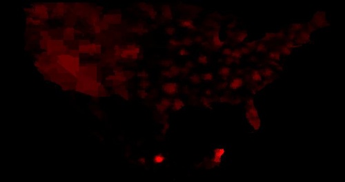
The Mexico/USA H1N1 Scenario was created in the early spring of 2009 as a first attempt to measure the basic reproductive number, Ro, of the H1N1 virus. Little biosurveillance data was available but we knew that the first 10 people had been reported with H1N1 in NYC. At this time there were approximately 6000-7000 cases reported in Mexico City.
The Scenario makes use of STEMs model for air travel (calibrated against FAA data). The basic scenario was run repeatedly using a range of values for the transmission rate. For each run, we compared the number of people infectious in Mexico city at the time 10 people first appear with H1N1 in NYC. From this work we estimated Ro~1.7
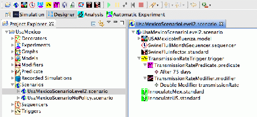
The downloadable project contains this basic model without any expressed policies. The project also contains a second scenario that shows how to set up Modifiers, Predicates, and Triggers. In this case the Modifier changes the transmission rate based on a time trigger.
Global Earth Science Models
This downloadable project contains re-useable continent-level models of Earth Science Data including
- elevation
- rainfall
- temperature and
- vegetation coverage (NDVI)
Please note: You need to access the STEM update site and install the "STEM Earth Science Data for 2010" plugin to use these models.
Instructions for adding this and other additional features may be found on the STEM Installation Guide.
Global Geographic Models Only
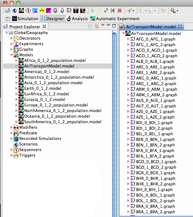
The Global Geographic Models project contains no runnable scenarios. Rather, is contains a set of pre-composed models for large regions of the world intended to be built upon in developing your own scenarios. These models, shown int he figure below, include a model for global air transportation, and a set of continent and super-continent models for geographic regions and people. After you download them, please expand them to see the inner components.
Super-Continent Examples
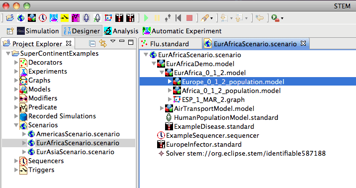
The Super-Continent Scenarios provide an examples of how to construct scenarios using the Global Model examples described above. These scenarios show how to model large regions such as the Americas, Europe+Africa, and Europe+Asia. The figure below expands the Eur-Africa Scenario. Note that the Inner Eur-Africa Model contains a model for Europe, a model for Africa, together with the connection between Spain and Morocco.
Chicken Pox
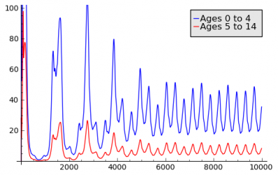
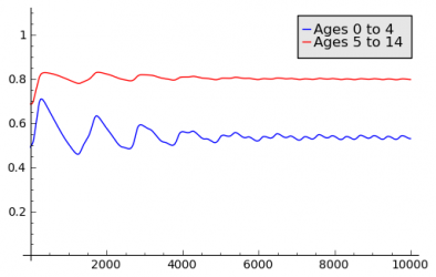
The Chicken Pox Scenario was created as an attempt to model a disease with lifelong immunity. An Aging Population Model is used to capture the different fractions of immune people for different age groups. Immunity acquired in one age group has an influence on the following age groups, since immune people age into these groups. Seasonal variations are achieved by using a Seasonal Population Model based on Interpolation of Sampling Points. The models are applied to geographic model of France. The following charts show the results for incidence and fraction of immune people for two different age groups.


