STEM Population Models

Models of Population

Disease spreads through populations in many ways. In order to model complex zoonotic and/or vector borne disease models one needs to be able to simultaneously model multiple populations. STEM provides a framework for this. For more information on modeling the diseases themselves, please see the page on STEM Disease Models.

Basic Models

Standard Population Model

The standard population model can be used to model a population that growths or shrinks by a background birth rate and death rate. It is commonly used to model basic human population dynamics. For human populations, the STEM provides census data to initialize the populations base on real census data. These populations can be held fixed or adjusted based on birth rates, death rates and the time/date of your simulation.

Advanced Models

Mosquito Population Model

The mosquito population model in STEM uses environmental earth science data (available in the STEM library) to estimate the average mosquito population for a region. Our goal is to compute temporal and regional probability for presence of mosquitoes from environmental variables. If we assume that the mosquito probability at time t and location r follows a Poisson distribution, and if the density depends on independent variables describing or defining the local environment at (t,r), then the logarithm of the expected value for the (un-normalized) probability can be expressed as a linear combination of the independent environmental variables (Charoenpanyanet 2009, Cameron 1998, Christensen 1997):

P(t, r) = kP(T, t, r)*P(R, t, r)*P(V, t, r)*P(E, r) (Equation 1)

Suppressing the space and time variables (t,r), P(T) represents the temperature dependence, P(R) represents the rainfall dependence, P(V) represents the NDVI dependence and P(E) the elevation dependence. If any of functions is zero, then the joint probability is also zero. By expressing the total risk as a joint probability distribution based on a product of environmental functions, we can normalize or rescale the expected mosquito probability using a single population calibration constant k. This calibration constant is chosen such that the value of P is calibrated to the observed mosquito burden.

In Equation 1, the temperature factor P(T) uses average night time surface temperature (Celsius). Daily mosquito survival p (assuming constant humidity) is defined as (Martens 1997):

(Equation 2)

Another temperature dependent variable is the larval duration ld (Jepson 1947):

(Equation 3)

We define our temperature factor P(t) as the combined effect of ld and p (Craig 1999):

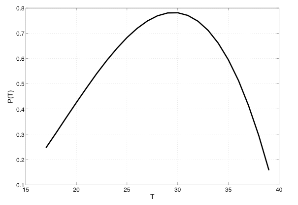
P(T) = (-4.4+1.31T-0.03T^2)*(0.00554T-0.06737) (Equation 4)

If the temperature is less than 16 C or greater than 40 C, we set P(T) to zero. This figure shows a plot of P(T) versus temperature T:

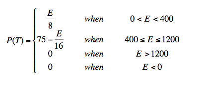
The elevation factor in Equation 1 uses altitude above sea level in meters. Field studies of Anopheles in Thailand along with remotely sensed elevation data in both wet and dry seasons suggest Anopheles population size is strongly peaked at an elevation of ~400 meters (Charoenpanyanet 2009). We parameterize the Thailand observations with an elevation function that increases linearly from 0-400 meters, and falls linearly from 400-1200 meters, and is zero above 1200 meters.

(Equation 5)

The dependency on rainfall P(R) is based on mosquito density surveys. In a rural town in western Kenya, the average number of blood fed An. Gambiae and funestus mosquitos per house was measured (per month) between October and May 2000 (Okara 2010). The data suggest an approximately linear relationship between mosquito population and rainfall level. Hydrologic studies suggest rainfall leads to increases in standing water necessary for larval growth. We model P(R) with a simple linear approximation:

P(R) = R(t, r) (Equation 6)

where R(t, r) is the monthly average rainfall (mm) at location r and time t.

The vegetation factor P(V) is based on the Normalized Difference Vegetation Index (NDVI). The NDVI algorithm used in the TERRA/MODIS mission is described in detail by (Huete et al. 1999). The NDVI scale ranges between -0.1 and 0.9 where -0.1 represent bodies of water; values close to 0 correspond to sand, rock, desert or snow; and values between 0.2 and 0.4 represent shrubs and grassland. NDVI near 0.8-0.9 corresponds to tropical rainforests or other forested areas with high density of green leaves. NDVI changes seasonally and over longer time scales with global climate change and deforestation.

A field survey of 26 sites in Thailand measured the dependence of mosquito density on NDVI, as determined by the number of female mosquito bites per person-hour (Charoenpanyanet 2009). A survey in South Korea showed the effect of NVDI on the local density of larvae (Rueda 2010). In both studies, the mosquito population was found to be approximately zero below NDVI <0.3, and to increase approximately linearly for NDVI > 0.3. Based on these works we approximate the vegetation factor as:

(Equation 7)

Our model for Malaria transmission (see below) depends on an estimate of the actual number of mosquitoes in a region. We assume that female Anopheles mosquitoes feed exclusively on humans (no malaria reserve is assumed in animal populations). So if no humans inhabit an area, no mosquitoes can survive. Furthermore, we assume a mosquito travels at most 50 meters in search of a blood meal, so if the human areal density is less than 127 people/km2 (1 person in a 50 meter radius circle), mosquito survivability is reduced.

Our estimate for the number of (female) mosquitoes in a region, N(t, r) , is:

where A(r) is the area (in km^2) for region r, is the human population density of region (in humans/ km^2). Observe that in this case, the scaling factor k in Equation 1 is calibrated to observed mosquito areal density.

References

Charoenpanyanet A (2009) Anopheles Mosquito Density Predictive Model Based on Remotely Sensed Data. Doctoral Dissertation Asian Institute of Technology, Bangkok, Thailand

Cameron AC, Trivedi PK (1998) Regression Analysis of Count Data. New York: Cambridge University Press.

Christensen R 1997 Log-Linear Models and Logistic Regression, 2nd edn. New York: Springer-Verlag.

Martens WJM, Jetten TH, Rotmans J, Niessen LW (1995) Climate change and vector-borne diseases. Global Environmental Change, Vol 5. No. 3. pp. 195-209, 0959-3780(95) 00051-8

Jepson WF, Moutia A, Courtois C (1947) The malaria problem in Mauritius: the bionomics of Mauritian anophelines. Bull. Entomol., Res. 34, 89

Craig MH, Snow RW, le Seue D (1999) A climate-based sistribution model of malaria transmission in Sub-Saharan Africa. Parasitology Today, vol. 15, no. 3.

Huete A, Justice C (1999) MODIS VEGETATION INDEX (MOD 13) Algorithm theoretical basis document (http://modis.gsfc.nasa.gov/data/atbd/atbd_mod13.pdf)

Rueda LM, Brown TL, Kim HC, Chong ST, Klein TA, Foley DH, Anyamba A, Smith M, Pak EP, Wilkerson RC (2010) Species composition, larval habitats, seasonal occurrence and distribution of potential malaria vectors and associated species of Anopheles (Diptera: Culicidae) from the Republic of Korea. Malaria J 9:55. doi:10.1186/1475-2875-9-55.

Seasonal Migratory Population Model

Figure 1: An example square lattice scenario demonstrating how to create a model of migratory birds is available on the scenarios page

The Seasonal Migratory Population Model works together with the Seasonal Migration Edge Graph Generator or a sub-graph of migration edges appropriately designed. It allows users to create models where animals migrate seasonally between regions. The edges are just ordinary migration edges. The Migratory Population Model simply modulates the migration rate with a sinusoidal function. As such, negative migration rates are simply ignored by the population model and the population moves only along edges with positive rates. At the end of the season, when the sign of the migration rates changes on some nodes, so does the direction of migration. The Seasonal Migration Edge Graph Generator is a simple way to create a suitable collection of migration edges between two regions. Users are free to create their own sub-graph by other means including pajek. In the downloadable example available on the scenarios page, we show how a migratory sub-graph was constructed for an existing square lattice.

Multipopulation Models

Demographic Population Model

The Demographic Population Model allows to divide the whole population into groups. This can be useful to model disease it must be distinguished between men and women, children and adults etc.. The model is based on the Standard Population Model, so the population growths or shrinks by a background birth rate and death rate. Please see the documentation on Using Structured Populations in STEM.

Aging Population Model

This model is an enhancement of the Demographic Population Model. It allows to divide the population into groups regarding the people's age. The process of aging is also implemented, which means that fractions of each age group move to the respective next age group as time passes. Additional documentation may be bound on the tutorial page Using Aging Populations in STEM.