Notice: This Wiki is now read only and edits are no longer possible. Please see: https://gitlab.eclipse.org/eclipsefdn/helpdesk/-/wikis/Wiki-shutdown-plan for the plan.
2019 novel Corona Virus Model
The 2019 novel Corona Virus (nCoV) Model is an all in one archive available on the download page that allows you to install and run a global model to study 2019-nCoV.
Please Observe: The precise epidemiological parameters are not known at this time. The downloadable scenario can be used to see how
changes to the parameters changes the spread.
What Sars-CoV-2 Models are available?
There are now three different corona virus models available available for stem.
The first, a simple model named  ncov.eclipse.org.coronavirus  comes with a pre-built global scenario
designed to study interventions restricting international air travel. This model we build in January 2020.
Since that time local community spread is occurring throughout the globe with the growing corona virus pandemic.
In order to appropriately model that spread it is essential to capture transmission from Asymptomatic individuals.
The new model, Sars-CoV-2b, captures asymptomatic transmission. It comes with a  scenario designed
with a single graph node that can be used for fitting model parameters from outbreak from any local region
(eg county, state, or country).
A few words about Case Reporting Rates
Two of the models described on this page use a parameter named the Case Reporting Rate partition new incidence across two paths (symptomatic infectious and asymptomatic infections). The term itself suggests that asymptomatic cases are not reported where-as symptomatic cases are, however there is nuance that must be considered. In reality, incidence that follows the asymptomatic path should be understood simply as not reported incidence. This includes cases that were truly asymptomatic, cases with symptoms so mild as to not result in an clinical encounter, and/or errors in reporting. In this sense the A compartment includes all non-reported incidence.
Please also remember that an underlying assumption of epidemiological compartment modeling is that the population in a region being modeled is well mixed. If you construct a model where a very large region is treated as one well mixed node this can result in errors. For example, if you create a patch model for the world where a large country like China is treated as one well mixed patch (e.g., modeling at admin level 0 instead of state or county). The model puts entire population of China in that one patch. But, if the actual epidemic in China is concentrated in one region or city, that scenario has a built in error. Since the entire population is not well mixed, the denominator in the mass action term should be the population of the affected province or city - not the whole country. In fitting the city reference data (as if it represents country data) the solver will compensate by decreasing the "Case Reporting Rate" to an unrealistically low value. The fix is to model at higher spatial resolution. Country level modeling can be useful for small country's but keep in mind the underlying well mixed assumption if composing your scenario at low resolution.
(new) Advanced SACIR(S) model capturing Asymptomatic Transmission
Archive and it's contents
The archive contains two folders. Both of these components must be imported directly into your STEM work space (not nested in another folder).
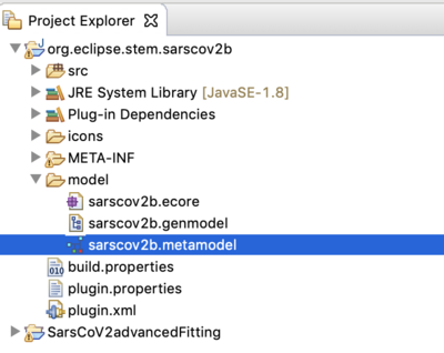
- The project org.eclipse.stem.sarscov2b is the model builder project containing the disease model.
- To see the model itself, from the designer perspective, double click on the .metamodel file in the model sub-folder.
- Project folder SarsCoV2advancedFitting contains the single node scenario and automated experiment needed to fit the model to data.
Getting the Downloadable Scenarios
Please visit the downloads page and download the model.
Please see: Importing and Exporting Projects
Extract the archive to your local file system. It contains two primary components. The model builder project org.eclipse.stem.sarscov2b, and a run time example project SarsCoV2advancedFitting
Setting up the model
Once you have imported both projects and can see them all, un-nested, in the project explorer (in your workspace),
- navigate to the org.eclipse.stem.sarscov2b
- open the models folder.
- make sure you are in the designer perspective
- double click on sarscov2b.metamodel
- you should the see the compartment model itself as shown below.
- After importing the scenarios you may also click the gear icon in the model builder to recompile all the generated Java code and plugins (this is only necessary on some systems, but it's a good idea to do it on import.
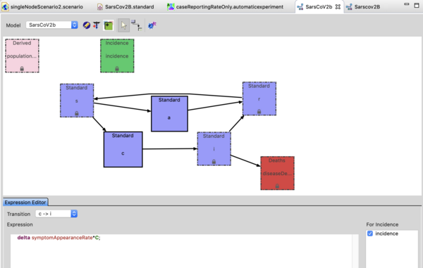
The Sars-CoV-2 (b) model is an SACIR model where A represents individuals who are shedding virus (infectious) but asymptomatic.
The 'C' compartment represents pre-symptomatic individuals. This is a lot like an exposed compartment but in this case pre-symptomatic may also be shedding virus. The I compartment represents individuals who are infectious and symptomatic. The incidence by default is set to the transition from C -> I, as public health does not detect cases until they are symptomatic (I). In principle incidence is represents time of infection but there is a time lag in reporting (the difference between S -> C and C -> I). Click on the transition and see the expression in the expression editor. You can change which transition defines incidence simply by the checkbox to the right of the expression editor. Remember to regenerate if you do that. You can watch the youtube video on the model builder to see how this works.
- Navigate to the SarsCoV2advancedFitting project,
- open the decorators folder,
- and double click on the disease model (not the infector) to open it in the resource window. The disease model is a little black icon with a caduceus (the symbol of medicine). The black and green icon represents and initializer that reads the initial conditions form a sub-folder in the Recorded Simulations' folder
- Click on on the disease model in that window and open the property view below.
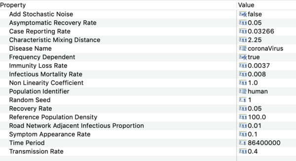
You should see all the parameter values defined in this model as shown in the image below.
Precise values are not known at this time. The settings used in the downloadable scenario are based on estimates from fitting the (public) reference incidence data for a metropolitan region. That data is included in the Reference sub-folder in the Recorded Simulations' folder.
Click on the transition from S -> C. Look at the expression editor. Click on the transition from S -> A and at the expression editor. Note that A, C, and I all contribute to the total infectious count. Also note there is only on transmission rate used. You can use the model builder to add separate transmission rates for contacts from the A,C, and I compartment - but be careful. With three parameters and limited data you risk over fitting.
Structure of the project
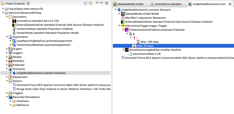
The SarsCoV2advancedFitting folder is a STEM project containing a number of components. If the screen shot below several of these sub-folders are open. Click on the decorator folder. It contains and instance of the disease model, an External Data Initializer, A population initializer (to set the human population in the region of interest, an a standard Human Population Model =br/>
The Experiments folder contains two automatic experiments (These will be discussed below).
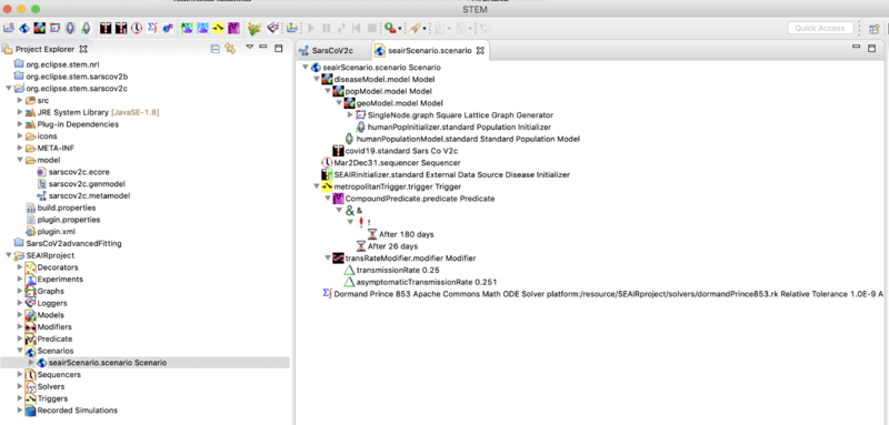
The Scenario folder contains the single node scenario designed for fitting case report data from a region. If you double click on it, the scenario will open in the resource set, that's the big window to the right. Open it to see the components of a scenario.
It contains objects from the project sub-folders which can be dragged and dropped into the scenario. You can also delete them from the scenario but you don't lose them form the project (so they can be added again). For example, from the projects decorators folder double click on the ExternalDataInitializer to open in the resource set. Select it and look in the Properties View (tab below). You can see that it is configured to initialize each of the SACIR compartments from the folder Recorded Simulations>initializers. Go to that folder to see the files it is using. If you want to model a different region from the metropolitan area provided as an example, you would have to edit or replace these files. Please see a discussion below.
Next open the project folder labeled Triggers. You can see the trigger in the scenario to the right. Triggers contain a Predicate and a Modifier. Triggers,Predicates, and Modifiers define STEM Interventions
You can define multiple interventions and add them to or remove them from the scenario. The example shown lowers transmission rate to 0.26 after 20 days, and returns it to the value in the disease model after 180 days. You may ask "20 days from what"? From start. If you look at the components of the scenario you will see a sequencer. This one is names Mar2Nov1.sequencer. Open the Sequencer folder in the project, double click the sequencer and it will open in the resource set. Select it and you will see the sequencer start and top dates in the properties view below.
Finally you can see the Scenario has a solver. In this case it's a Dormand Prince 853 solver. There are many to chose from and you can create several and drag them into your scenario (but remove remember to the old one first!).
Setting up the Initializer
The >Recorded Simulations>initializers folder contains six files. All six are required for this model. One file is name Population Count_0.csv and 5 other CSV files one for each compartment S,A,I,C, and R. The _0 indicates these files should decorate the top node in this graph. This is a single node graph so its level 0. In a county level 1 is a state, level 2 is county, etc. Note you can decorate the single graph node with any level regions you like (eg county down to city) the _0 does nothing in this case. If you open the file Population Count_0.csv you will see the following.
iteration,time,stem://org.eclipse.stem/node/6BE870A7261569D/LAT_SQR_0_0
0,3/2/20 12:00,8623000
1,3/2/20 12:00,8623000
There is a label for three columns. iteration, date (or time), and the url of a node in the graph. In this case we have only one node and that is it's unique identifier. You can go to the graphs folder, expand the graph, and find that url using the properties view.
The rows below show you can list several iterations or start dates. The External Data Initializer specifies which line to read at start. You could have several lines and just change the row number set in the initializer for the initializer should use. The value in the third column is the (initial) population to place in the location specified by the url. Let's call this population value P.
How to set the other values? Lets assume for a moment that there are no infections cases. Then we would only have to set S and R. In general, even if a disease is totally new, there is some herd immunity or inital resistance to the spread of an infectious disease in a population. For seasonal influenza that might be 20% or 30%. In pandemic, most but not all people are initially susceptible. In this example the initial herd immunity was set at 30% and the initial susceptibility at 70% so initially we might start with
S = 0.7*P
and
R = P-6
We didn't write R=0.3*S because you might want to make S an integer.
Now what about A,I,C? Well trivially you might think that I at time 0 is just 1 (so we will set time zero to the data a first case is reported). Howver, the date public health knows about first symptomatic case there might be many others they don't know about. In this example a start date was chosen with just 1 case but we initialized with 100 for this area with over 8 million people. You can/should do a sensitivity analysis around any number you start with. For now though let's just say I = 100. The value you use for C depends on the symptomAppearanceRate (which sets the rate people more from C to I), and the doubling time of the disease.
We used C = 1.2*I in this example.
The initial value for A depends in part on the ratio of Asymptomatics (A) to Symptomatics (C and I). For Corona Virus the Asymptomatics may be as high as 80-95% of the cases. You can try different values in the disease model and should do a sensitivity analysis on the multiplier k you use to get A.
A = k*(C+I)
Running the model (for the first time)
Before you try to run the model, navigate to the command bar ....
- On a mac go to >STEM>Preferences>STEM>Simulation Management one windows >Windows>Preferences>STEM>Simulation Management
- un-check scenario caching
- set the time delay to about 150 msec
Then navigate to
- Preferences>STEM>Solver
- and increase worker threads if you workstation has more than two core (for example 4 threads will help performance).
Remember you are about to load a global simulation.
- Open the Scenarios folder
- Select the singleNodeScenario2.scenario Scenario.
- Right click and click STEP the little foot step icon. (please do not click run yet)
- You should see a single square in the Graph Map view. This is a single node scenario representing (any) single location. Double click on the square to launch a time series monitor below.
- Hit run to run for the duration set by the sequencer.
Fit to Data with using Automated Experiments
STEM provides a Nelder-Mead downhill simplex algorithm to automate exploration of parameter space and minimize the normalized root mean squared error (nrmse). Please see the page entitled Running an Automated Experiment for more information.
Location of Reference Data
In the project explorer, open the folder >Recorded Simulations>Reference to see the reference data.
Please note, you have to provide the reference data. When you create the automated experiment you define the path to
the reference data so you can put it somewhere else but it must contain a file for incidence data and for population
data, both vs time. The structure is much like the structure for the initializers discussed  above.
AI Algorithm to find parameters that fit reference (daily incidence)
Navigate to the experiments folder in the project explored, open it, and double click on the 'CaseReportingRateExpt.automaticexperiment' to open it in the resource set (the big window to the right). Select it in the source set to expand it and show all components inside. Note that this experiment has one Modifiable Parameter: Case Reporting Rate. You can create experiments that modify more than one parameter at time. It is often very useful to have experiments designed to explore different sets of parameters (sometimes several and sometimes just one). If your parameter values are very far from correct (i.e. very far from the global minimum) the algorithm can get stuck in a local minimum. See the doc on Running an Automated Experiment for more information.
Note that every Automated Experiment contains a scenario. You select the scenario when you create the experiment. Scenarios are executable.
So are Automated Experiments. In fact these experiments run the enclosed scenario multiple times to explore parameter space.
- Click on the Modifiable Parameter: Case Reporting Rate and select the Properties view tab in the window blow. Click on the initial value an set it to 0.05 (which actually moves it was from the optimal value.
- Next select the 'CaseReportingRateExpt.automaticexperiment' in the project explorer, right click, and select run.
- Your application will switch to a new perspective (the Automatic Experiment Perspective). Look at the upper right hand corner and you will see the icon for this perspective looks like a little erlenmeyer flask with a 'A' in the upper left corner.
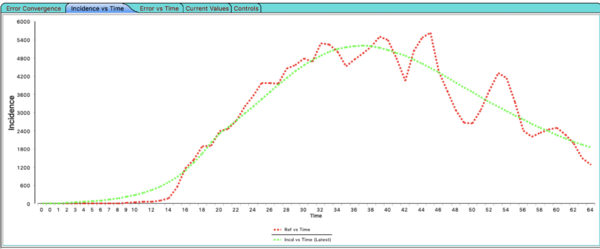
The Nelder-Mead algorithm as already stopped running by the time you read this. Click on the tab in the Automated Experiment window labeled Incidence vs Time. You will see the best (minimum nrmse) model output for incidence plotted along with the reference data.
The automated experiment will only fit over the time range of the reference data you provide - even if your sequencer
is configured to run for more iteration. It will only fit for the locations and times where reference data exists. This experiment
has a single node scenario so there is only one incidence file, one resolution (_0) and one location or node in the graph.
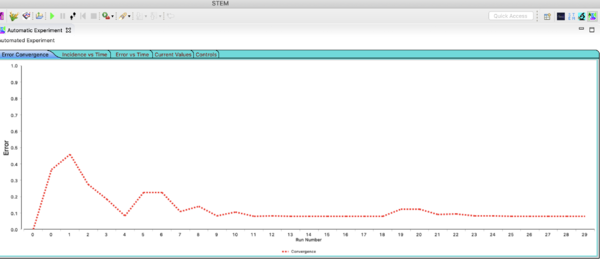
Next click on the tab in the Automated Experiment window labeled Error Convergence. You will see how the error changed in time with each set of parameter values the Nelder-Mead algorithm ran. Each point represents a different run of the simulation with a different set of parameter vslues (in this case the CaseReportingRate). After finding an minimum the algorithm restarts with a slightly different initial conditions. Thats why the red curve goes up again. It is checking that it was not trapped in a local minimum. The further the starting values are from the 'best' values, the more iterations will be run. Fitting more parameters at once will also increase the number of runs.
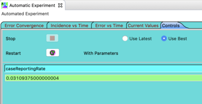
Next click on the tab in the Automated Experiment window labeled Controls. If the run is too long or not converging (e.g. because the initial values are too far off), this view proves a stop button. It also shows the current parameter value(s). Note the button labeled restart. After finding a minimum you can press this to trigger even more exploration of the parameter space. As Nelder-Mead walks around parameter space it is also reducing the step size. In principle restarting can provide more accuracy. In practice it's usually not necessary (but there is no harm in doing it).
Observe: Restart is a feature that requires the Automated Experiment to cached it's values. That means the disease (or population) model
parameter values cached in memory may not be the same as the persisted values defined in your disease model decorator. Why does this matter?
Suppose you are fitting several parameters and you decide you started with the wrong transmission rate. If you go back to you disease model
and change the transmission rate the Automated Experiment will not see the change between runs. If you find yourself changing parameter values
and the Automated Experiment is not responding to those changes - this is the reason. The solution is to restart STEM. We have a feature request
to provide a 'reset' button but at the time of this documentation that has not yet been implemented.
Note the radio buttons labeled use latest and use best. Select use best and go to the steps below.
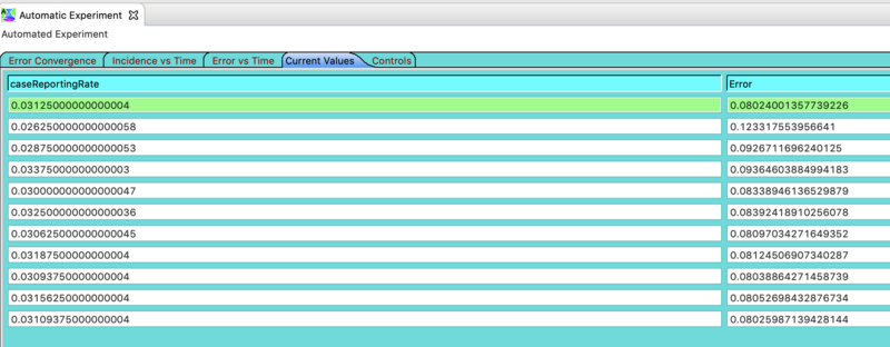
Click on the tab in the Automated Experiment window labeled Current Values. Here you can see all the values that Nelder-Mead explored along with the NRMSE obtained with that set of values. If you selected use best the best fit is on top. use latest is often the same best fit value (but not always). These values are also logged in the AutoExpTempDir in your workspace - but this log folder is not a STEM project so you won't see it in the project explorer. You'll have to look in your file system with Windows Explorer or Mac Finder.
Please Note: The Automated Experiment does NOT change you disease model settings. If you want to use the best fit parameters values it finds you will have to
edit your disease model by selecting it in the decorators folder and changing the value in the properties view.
Fitting disease deaths
Please see the documentation on Epidemiological Parameters and in particular this useful approximation and this general analysis.
Typically the infectious mortality rate, δ, represents single constant rate at which infected people die. If infected people stayed infected forever they would all eventually die because δ is a rate (with units of inverse time). Of course this does not happen because there is also a recovery rate and most people recover first and never become case fatalities. So there is a difference between the Case Fatality Rate which represent the total fraction of cases that become fatalities and the infectious mortality rate which has units of inverse time.
If you are using the graphical model builder you can define a more complex function defining the instantaneous infectious mortality rate (for example it may depend on availability of clinical care), but let's assume you are starting with a constant rate. In that situation calibrating the death rate is straight forward. You should do this after you have calibrated the daily incidence as described above.
- From the reference data you placed in your Reference folder, look at the Population data. From the delimited population data vs time make a delimited file with cumulative deaths vs time. Deaths start at zero and when population goes down cumulative deaths increase. Do population[time=0] - population[time=finish] represents total cumulative deaths. If you created a logger and have logged the deaths compartment you can do a least squares fit between predicted and reference cumulative deaths, or if you just want an a approximate calibration compute the total reference/predicted cumulative death ratio. If your death rate was low this ratio will be greater than one. If high, it will be less than one. Simply multiply your infectious mortality rate by this ratio.
(new) Advanced SEAIR(S) model capturing Asymptomatic Transmission
Archive and it's contents
The archive contains two folders. Both of these components must be imported directly into your STEM work space (not nested in another folder).
- The project org.eclipse.stem.sarscov2c is the model builder project containing the disease model.
- To see the model itself, from the designer perspective, double click on the .metamodel file in the model sub-folder.
- Project folder SEAIRproject contains the single node scenario and automated experiment needed to fit the model to data.
Getting the Downloadable Scenarios
Please visit the downloads page and download the model.
This downloadable package contains an example using the new compound error function. For more information on Automated Experiments please see the documentation on automated experiments
Extract the archive to your local file system. It contains two primary components. The model builder project org.eclipse.stem.sarscov2c, and a run time example project SEAIRproject
Setting up the model
Once you have imported both projects and can see them all, un-nested, in the project explorer (in your workspace),
- navigate to the org.eclipse.stem.sarscov2c
- open the models folder.
- make sure you are in the designer perspective
- double click on sarscov2c.metamodel
- you should the see the compartment model itself as shown below.
- After importing the scenarios you may also click the gear icon in the model builder to recompile all the generated Java code and plugins (this is only necessary on some systems, but it's a good idea to do it on import.
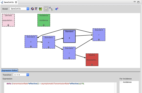
The Sars-CoV-2 (c) model is an SEAIR model. The 'E' compartment represents exposed individuals who are not yet infectious. The A compartment represents individuals who are shedding virus (infectious) but asymptomatic and the I compartment represents individuals who are infectious and symptomatic. The incidence by default is set to the transition from E -> I, as public health does not detect cases until they are symptomatic (I). Click on the transition and see the expression in the expression editor. You can change which transition defines incidence simply by the checkbox to the right of the expression editor. You could select S=>E but then incidence would include asymptomatics (who are not know by public health without comprehensive testing). Remember to regenerate if you do that. You can watch the youtube video on the model builder to see how this works.
- Navigate to the SEAIRproject project,
- open the decorators folder,
- Click on on the disease model in that window and open the property view below.
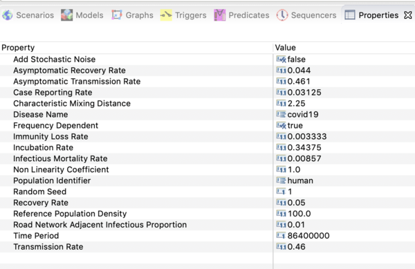
You should see all the parameter values defined in this model as shown in the image below.
Precise values are not known at this time. The settings used in the downloadable scenario are based on estimates from fitting the (public) reference incidence data for a metropolitan region. That data is included in the Reference sub-folder in the Recorded Simulations' folder.
Click on the transition from S -> E. Look at the expression editor. Note that A, and I both contribute to the mass action term. Also note there are two transmission rates used. You can set them to the same value or use different values but remember that reproductive number depends on a ratio of transmission rate to recovery rate. You can use the expression editor to change the parameters used by the model. Remember to regenerate the code if you do.
Structure of the project
The SEAIRproject folder is a STEM project containing a number of components. If the screen shot below several of these sub-folders are open. Click on the decorator folder. It contains and instance of the disease model, an External Data Initializer, A population initializer (to set the human population in the region of interest, an a standard Human Population Model. The structure is very similar to the structure decribed for the Advanced model above.
Setting up the Initializer
The >Recorded Simulations>initializers folder contains six files. All six are required for this model. One file is name Population Count_0.csv and 5 other CSV files one for each compartment S, E, A,I, and R. The _0 indicates these files should decorate the top node in this graph. This is a single node graph so its level 0. In a county level 1 is a state, level 2 is county, etc. Note you can decorate the single graph node with any level regions you like (e.g., county down to city) the _0 does nothing in this case. If you open the file Population Count_0.csv you will see the following.
iteration,time,stem://org.eclipse.stem/node/6BE870A7261569D/LAT_SQR_0_0
0,3/2/20 12:00,8623000
1,3/2/20 12:00,8623000
The process of setting the initial values is very similar the process described for the model above.
Running the model (for the first time)
Please see the steps described above.
Fit Data with the Automated Experiment
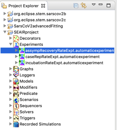
In the Project Explorer, open the Experiments folder in the SEAIRproject folder. You will see that the project comes with several experiments.
- Please see the documentation for the advanced model above for examples of data fitting. The steps are essentially the same.
- See the section above regarding the location of reference data
- See the section above regarding finding parameters with reference daily incidence
- Try to create you own experiment.
Simple Global Model with Air travel
Archive and it's contents
The archive contains four folders. All four of these components must be imported directly into your STEM work space (not nested in another folder). If you already have the GlobalGeography or the SuperContinentExamples projects installed you need not reinstall them (but they are required to run the scenario).
- The project ncov.eclipse.org.coronavirus is the model builder project containing the disease model.
- To see the model itself, from the designer perspective, double click on the .metamodel file in the model sub-folder.
- Project folder CoronaVirus contains the global scenario.
Getting the Downloadable Scenarios
Please visit the downloads page and download the 2019 nCoV model.
Extract the archive to your local file system. It contains four primary components.
Setting up the model
Once you have installed all four projects and can see them all, un-nested, in the project explorer (in your workspace),
- navigate to the ncov.eclipse.org.coronavirus
- open the models folder.
- make sure you are in the designer perspective
- double click on coronavirus.metamodel
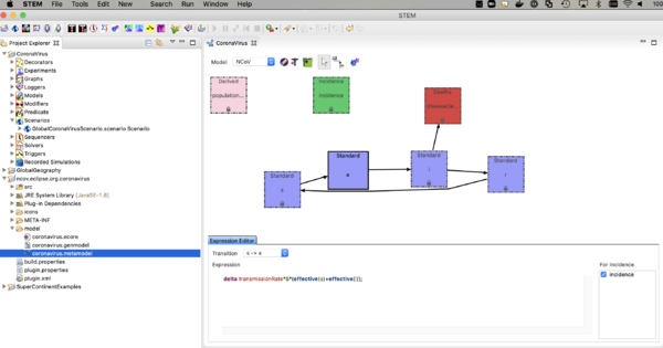
- you should the see the compartment model itself as shown below.
- After importing the scenarios you may also click the gear icon in the model builder to recompile all the generated Java code and plugins (this is only necessary on some systems, but it's a good idea to do once on import.
The nCoV model is an SAIR model where A represents individuals who are shedding virus (infectious) but asymptomatic. The I compartment represents individuals who are infectious and symptomatic. The incidence (or transition from S -> A, depends on the sum of the fraction infectious in both A and I. Click on the transition and see the expression in the expression editor. You can watch the youtube video on the model builder to see how this works.
The model looks a lot like an SEIR model but there is no incubation state (E) or incubation rate (you could add that if you want to). The reason to explicitly model the A compartment is that one can add interventions (predicates, modifiers, and triggers) based on the I state but not A. The rate individuals move from A -> I is called the "Symptom Appearance Rate" in this model. Next,
- Navigate to the CoronaVirus project,
- open the decorators folder,
- and double click on the disease model (not the infector) to open it in the resource window. The disease model is a little black icon with a caduceus (the symbol of medicine). The infector is the same symbol with a capital letter 'I' in one corner.
- Click on it in that window and open the property view below.
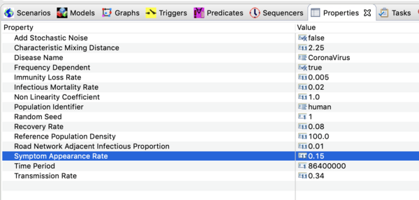
You should see all the parameter values defined in this model as shown in the image below.
Precise values are not known at this time. The settings used in the downloadable scenario are based on upper estimates for the basic reproductive number reported in the literature as of Jan 30, 2020. Ro depends on the transmission rate, β , the recovery rate, γ , and the infectious mortality rate, μ .
Ro = β/[γ + μ]
With the values shown above this puts Ro ~ 3.4. The first case appeared in mid December 2019. If you run the simulation for 45 days you will see the current settings over estimate cases in China but under estimate incidence from air travel. The high end estimate for Ro is likely too high and the build in STEM air travel model probably underestimates recent traffic.
Please Note: If you'd like to run the global simulation with one of the advanced models described above it is easy to do.
Just go to the models folder, open GlobalCoronaVirusModel.model, and delete the disease model from GlobalCoronaVirusModel.model
Import the project(s) above following the doc above. Then you can create an instance of either or both of these models.
It will appear in your decorators folder. Make sure to you use the same case sensitive disease NAME ("CoronaVirus" ) in
the new disease instance. Just drag the new instance into GlobalCoronaVirusModel.model and you are set to go.
Running the model (for the first time)
Before you try to run the model, navigate to the command bar ....
- On a mac go to >STEM>Preferences>STEM>Simulation Management one windows >Windows>Preferences>STEM>Simulation Management
- un-check scenario caching
- set the time delay to about 150 msec
Then navigate to
- Preferences>STEM>Solver
- and increase worker threads if you workstation has more than two core (for example 4 threads will help performance).
Remember you are about to load a global simulation.
- Open the Scenarios folder
- Select the GlobalCoronaVirusScenario.scenario Scenario.
- Right click and click STEP the little foot step icon. (please do not click run yet)
- Depending on your laptop you might want to get a cup of coffee. The model has been tested on a 2018 macbook pro and the global graph does load without error, but it will take a couple of minutes to load.
Once the map loads you can pan by clicking and draging the map and zoom with up and down arrows.
- Right click on the ocean and select a gain factor of 1,000,000
- Step a few more times until you are at about day 4
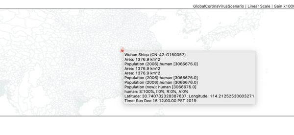
- Zoom in on China until you can find the red administrative zone where the infector seeded the first case(s). This is Wuhan Shiqu (Wuhan City).
- Double click on Wuhan to start a time series monitor for that region.
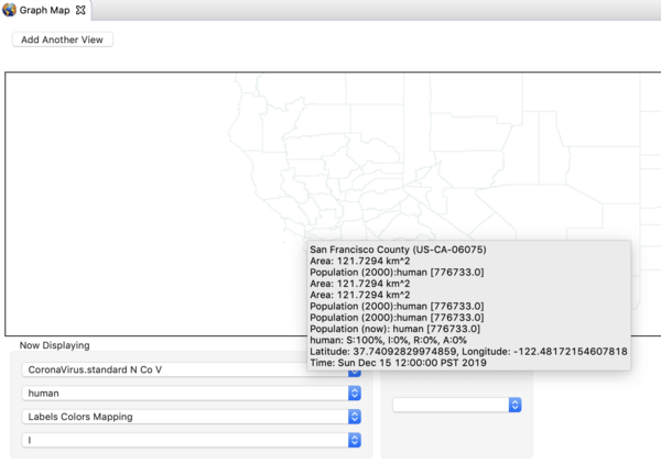
- Zoom and Pan until you find San Francisco in California, and double click to set up a monitor for that region.
- Right click on the map again and set the gain factor down to 1000. This is high enough to see the early cases.
- Click "run"
- When you get to about 50 days (Sequencer time Jan. 30) you might hit pause and then step again until you see evidence for infection via air travel.
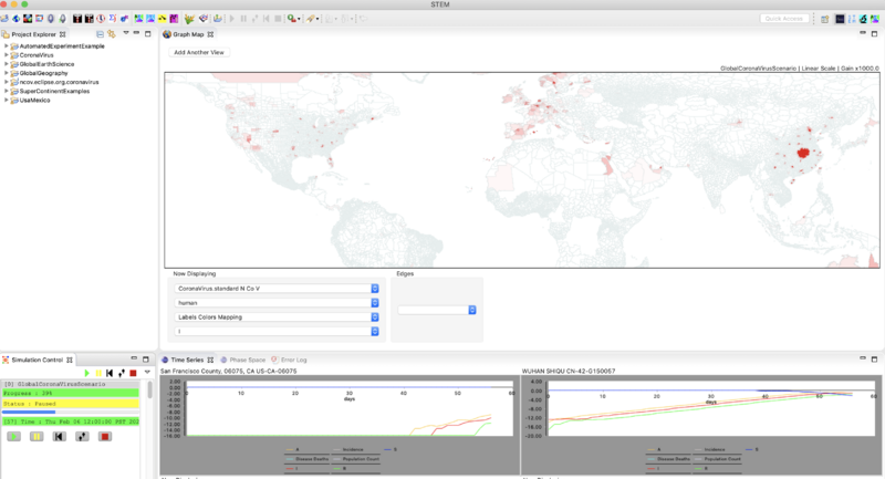
- At 57 days (Sequencer time Feb. 6) the simulation should look like this. Note that in the image below both time series monitors have been set to show a logarithmic scale (right click on the monitor to do that).
Next Steps
- Once you have the scenario running, go back to the property view for the disease model and see how changing the parameters effects the spread.
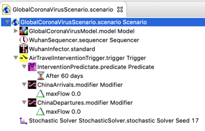
- As of Jan 31,2020 an example intervention has been added to the downloadable scenario. The new Scenario structure is shown below.
- In this example, the predicate is set to trigger the intervention at 60 days (so it does not change the behaviors described above). At 60 days, the edges regulating air travel two or from China are modified to set the max flow to zero for international travel. You can change this by changing the time parameter in the modifier. Please see the interventions documentation to learn about Triggering interventions in general.
Additional documentation
relevant to installing and running the model
Please see the following wiki pages for help
- Importing and Exporting Projects
- using the The STEM UI and Map View
- setting up Simulation Data Logging
- Triggering interventions
Please observe: Logging the simulation data from a Global scenario to a delimited file takes an enormous amount of memory
and should only be attempted when STEM is running on server (headless and with lots of  memory allocated to the heap).

Please see: Running STEM Headless

Please Also Note: There is a defect when logging compartments generated by the model builder.
For the workaround please see the page Server Side Logger Workaround
To test logging on a laptop please set up a smaller scenario with fewer countries. When logging on server please look at the buffer size setting in the logger object. You can adjust to buffer size to balance performance based on the memory available on your machine.
Acknowledgements
The STEM community would like to acknowledge Dr. Ira B. Schwartz, Navy Research Laboratory and University of Maryland, for the SEAIR model and Dr. Brian M. Gurbaxani(CDC/DDPHSS/OS/OTI) for suggesting the global air travel model.


