Notice: This Wiki is now read only and edits are no longer possible. Please see: https://gitlab.eclipse.org/eclipsefdn/helpdesk/-/wikis/Wiki-shutdown-plan for the plan.
Introduction to Compartment Models
Background
Please also see the page discussing the meaning and definition of common Epidemiological Parameters
Transmission of infectious disease in humans is a stochastic process. Whether or not a person susceptible to the flu in a given year actually contracts it is in large part a matter of chance. It is possible to become exposed by an infectious person shopping at the same supermarket – or to escape exposure based on the fortune of gathering goods in a different aisle. How can we do mathematical modeling of a process when its dynamics are subject to random events?
Jakob Bernoulli (1654–1705) was the first mathematician to prove a theorem known as the Law of Large Numbers [1]. In 1713, eight years after his death, his proof was published by another mathematician (his nephew Nikolaus Bernoulli) in a paper entitled The Art of Conjecturing (Ars Conjectandi) [2]. Bernoulli’s proof of the Law of Large Numbers is one of the most important theorems in probability and statistics. It demonstrates for a large enough system, the mean value of a random variable is stable over long periods of time or large numbers of samples.
Coin Flip Example
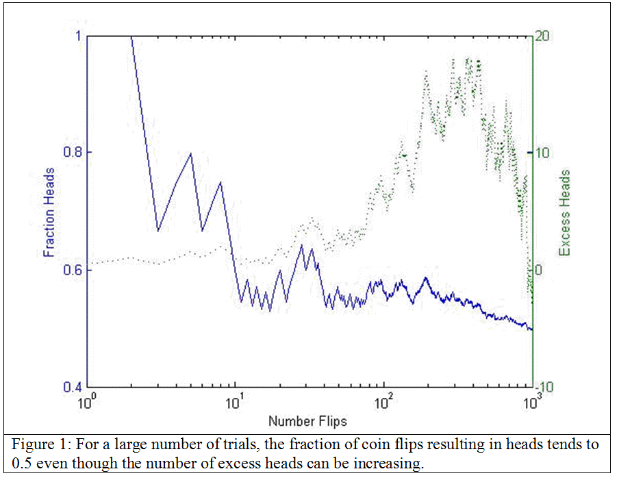
A useful example of this theorem is the outcome of repeated flipping of an unbiased or “fair” coin. An unbiased coin will land heads or tails with a probability of 50%. After a single flip,
the number of heads will be either zero or  one. This is not a good statistical sample as one would not want to conclude from a single trial that one expects to get a heads 0% or 100% of the time.
After a larger and larger number of trials, the average result will get closer and closer to 50%. After 100 flips, there might be 60 heads (10 excess) and after 1000 flips perhaps 520 heads (20 excess).
The number of excess heads would have doubled while the mean would have decreased from 60% to 52%, converging on the long-term stable value of 50%.
One of the earliest attempts to use the principles of statistics and probability to understand infectious disease was made by yet another member of the Bernoulli family. In a paper published in 1766,
Daniel Bernoulli used census data and statistical methods to study the advantages of variolation or variolization as inoculation against smallpox [3]. In a process originally developed in Asia,
smallpox scabs were dried, ground, and inhaled by people, who then contracted, hopefully, a mild form of the disease. Approximately 2% of individuals who contracted smallpox by variolation died compared
to 30% of those normally exposed to the disease.
The ability to study large numbers of cases and large populations makes possible the application of statistical methods to the study of infectious disease. In particular, we can make accurate predictions
using models based on continuous variables. Consider again the coin flip example. At any given point of time, by definition, a coin will be found in a particular state, heads or tails.
Imagine a collection of many thousands of coins being repeatedly flipped from one state to another. For a large population, P, the number of coins likely to be found in the heads state is simply:
Nheads=pheadsxP
where P is the total number of population of coins and pheads is the probability of a coin landing heads (pheads = 0.5). Compartment models are mathematical models designed to describe
the transport of information, material, energy, heat, etc., between and among the various compartments of a dynamic system. Formally, a dynamic (or dynamical) system is any system wherein objects interact
by a fixed set of rules or equations that describe the time dependence of the state variables of the system. For example, a system of planets orbiting a star is a dynamic system where the position of each
planet varies with time in accordance with Newton’s Laws of Motion. Compartment models were first introduced by Jay Wright Forrester who developed them for the field of Operations Research.
Forrester is credited as the father of System Dynamics.
Compartment models have been applied to the study of dynamical systems in fields as distinct as manufacturing (workflows), systems biology, environmental studies, economics, politics, engineering, and medicine.
First published in the Harvard Business Review in 1958 [4], Forrester’s work establishes a paradigm that can be applied wherever one wants to describe how a system changes in time.
What Is a Compartment Model?
A compartment model provides a framework for the study of transport between different compartments of a system. Think of each compartment as a room in a house. A person living in that house travels from room to room over time. At any given time the person may be found in the living room, the kitchen, the bedroom, etc. At no time will the same person be found simultaneously to be in two different rooms. Entities within a compartment model will exist in well defined states. “John is now in the living room.” There may be more than one person living in the house. “John and Jane are in the living room, Julia is in the kitchen.” If the house is a closed system so nobody ever enters or leaves, then summing the number of people in every compartment or room of the house will always yield the total occupancy of the house. In a closed system the number of people is conserved. If the system is open, the occupancy of the house might vary from time to time, but the number of people in a house, plus the number entering, minus the number leaving, is still conserved.
A house may have many rooms. In general, there can be a large number, N, of components and they may connected in different ways. It may be possible to enter the kitchen from the living room or from the dining room. Our coin flip example is a very simple model with two compartments. After any given flip of a coin, it is found to be in one of two states (either head or tails).
In medicine, compartment models have been used to study the dynamic flow of chemicals (nutrients, hormones, drugs, radio-isotopes, etc.) between different organs of the human body. The flow of material in a compartment model follows certain rule. (For a blood alcohol concentration of x%, alcohol a will pass through the blood/brain barrier at rate y mg/hour.) These rules, in turn, may be expressed as mathematical equations.
Perhaps the best reference to learn about he Epidemiological Compartment models defined in STEM is the book by Anderson and May [1].
SI(S) Models
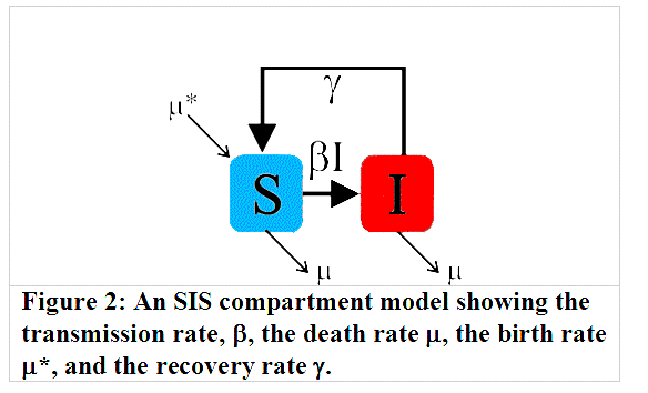
Similarly, models of the behavior of an infectious disease in a large population of people consider each individual as being in a particular state. These states are often called compartments, and the corresponding models are called compartment models. The simplest compartment models assume a person can be in one of only two states, either susceptible (S) or infectious (I). The two-state model is called the SI(S) model. Not all diseases are accurately described by a model with only two states, but a two-state model is useful in describing some classes of microparasitic infections to which individuals never acquire a long lasting immunity. Certain RNA viruses such as rhinoviruses and coronaviruses (the common cold) mutate so rapidly that individuals recently recovered from a cold will still be susceptible to other strains of the same virus circulating in a population. In a simple model for this process, individuals never enter a recovered state, but rather alternate between being susceptible and being infectious, just as a flipping coin alternates between heads and tails. Figure 2 illustrates a SIS model.
However, the process of infection differs from a random coin flip. In an SI model (or any standard compartment model), individuals move from the Susceptible state (S) to the Infectious state (I) by mixing or interacting with infectious individuals. If almost the entire population is Susceptible, then the rate of change in the number of Infectious people (Δ I) must be proportional to:
where β, the transmission rate, is also shown in Figure 2. This expression is, of course, incorrect for large numbers of infectious people because the total population is not always entirely susceptible to infection. Once there are no susceptible people left to infect, there can be no new infections. The correct expression is given by:
where the total population P = (S+I), and S/P is the fraction of the population Susceptible to infection. Equation 1a is an interaction term or interaction product because it represents the interaction between infectious people and susceptible people as a simple product. This interaction product, determines the new incidence of infection.
Rate Equations
The incidence corresponds to the number of new cases and would be proportional to the number of case reports that might be received by a state or local health department in the event of reportable disease. Incidence, however, is not the entire story. The number of infectious individuals over time includes people infected in the past, the new incidence of the disease, and decreases by the number of people who recover. Figure 1 shows that once people become infectious they eventually recover from the infection. If there is no long lasting immunity, they “recover” back into the Susceptible state. This process is modeled as a simple rate equation with a constant recovery rate y. The change in the number of infectious people (Δ I) in a given time interval is then:
where y has units of [people/time interval] or [people/day] for a time interval of one day. Often the expression in Equation 1b is sufficient for an accurate SIS model. However, if the recovery rate is sufficiently slow or the time intervals sufficiently long, it may be necessary to also include in the model the rate of births and deaths. Figure 2 shows how individuals from each of the state S and I can be removed from the population by a death rate:
Within this equation, the birth and death rates are taken to be equal if the population is approximately constant over the time of the epidemic. If the disease has a high mortality (for ex. HIV), a new parameter called disease related death rate (δ) can be assigned to track the deaths caused by the disease. In this case, the total mortality rate for infectious state is (μ + δ). When both the birth rate and death rate(s) are taken to be zero, the compartment model is said to be closed, i.e., the population is static with no new individuals coming or going. A compartment model with births, deaths, and/or a model including the spatial movement of people is said to be open. For a constant population with equal birth and death rates (μ*=μ), the SIS model is described by a pair of equations:
The pair includes two finite difference equations that predict the finite change in the number of people in each of the two states (I and S) over a finite or fixed time step. Using this pair of equations, with the total population, the transmission rate, the recovery rate, and the initial number of infectious people, we can obtain S(t) and I(t) over time (t).
If we assume the birth rate and death rate to be equal and therefore taken to be zero, equation 2 derives the number of people in each of the states S and I as a function of time. At t=1 (day), the population in S is simply the total population, i.e., the number initially infectious; the number of people in the S and I states is computed iteratively at each successive time step. In an SIS model, the recovery rate is not zero. Even though people are continually moving between the states S>I>S>I… and even though the simulation is initialized with only one infectious person, it is clear from the onset that both the Infectious and Susceptible populations, over a long enough period of time, approach a constant value equal to ½ the total population. This fixed point represents an endemic infection. In the SIS model, the infection is always circulating in the population. An infectious period of 5 days, for example, is the inverse of a recovery rate of 0.2 people/day.
The Reproductive Number
Whether or not a disease will spread throughout a population is determined by the Basic Reproductive Number,Ro. For an SIS model, Ro is the product of the infectious period and the transmission rate:
Ro = 5 x 0.4 = 2.0
When Ro > 1.0, the disease is infectious. When Ro < 1, the disease will die out. By implementing interventions that lower the transmission rate, public health officials can reduce the basic reproductive rate of a disease.
The Mass Action Term
The SI(S) model contains the important mass action term or interaction product,
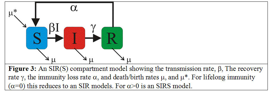
which describes how infectious people transmit an infection to susceptible people. However, not all infectious disease is well described by only two states. More generally, after exposure to microparasitic infection, individuals who recover from a disease will enter a third state where they are immune to subsequent infection. This Recovered State, R, appears in the SIR(S) compartment models, as shown in Figure 3.
For infections that confer lifelong immunity in the recovered state, an SIR model is appropriate. Typical examples for which an SIR model is used include Paramyxovirus (measles) and Viral Parotitis (mumps). In cases involving the Orthomyxoviridae viruses (which cause seasonal flu), immunity is not lifelong and may decrease over time. Immunity loss can reflect a decrease in an individual’s immune response, or a genetic drift in the circulating strain of virus that diminishes the effectiveness of the acquired immunity. In either case, an SIRS model represents the rate at which people in a Recovered state return to a Susceptible state at a rate α, the immunity loss rate.
The equations that define an SIR or SIRS model are shown in Equations <3> where now:
P = (S+I+R)
with α as the immunity loss rate, and the birth rate equal to the death rate.
In an SIR(S) model, the disease parameters include the total population, the transmission rate, the recovery rate, and the initial number of infectious people. It also includes the initial Recovered population, the number of people who are initially immune. Assume this number is initially set to zero and, as before, the birth rate and death rates are also taken to be zero. Below these constants, the number of people in each of the states S, I, and R is a function of time. At t=1 (day), the population in S is simply the total population – the number initially infectious. The new incidence is calculated from these two numbers, using Equation 2. From this term and the other terms in Equation 2, the number of people in the S, I, and R states is computed at each successive time step. Assume, for example, that the immunity loss rate is set near zero (α = 0.01). Since initially almost the entire population is susceptible, an epidemic wave results. Over long periods of time, the model still goes to a fixed point with a very low level of endemic infection. However, if the immunity loss rate had been set to zero (lifelong immunity), the infectious disease would have gone extinct since this is a closed compartment model.
The Recovered State, R, in an SIR(S) model is sometimes called the Removed state. This alternate name is appropriate as recovered individuals are immune in the model and therefore “removed” from the interaction term that leads to new incidence of infectious individuals (Equation 1a). If the immunity loss rate is non-zero, then Removed individuals become susceptible at a rate α. If we include a mortality rate m in each compartment, for an SIR(S) model, the basic Reproductive Number, Ro, is given by:
SEIR(S) Models
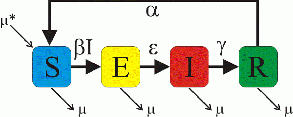
Many infectious diseases are also characterized by an incubation period between exposure to the pathogen and the development of clinical symptoms. If the exposed individual is not infectious during this incubation period (e.g., not shedding virus), it is important to model the incubation time explicitly. Note that there is a difference between an incubation time and a period of latency. A virus may or may not be dormant when an individual is in an exposed state. It is important to model the Exposed (E) state explicitly when there is a delay between the time at which an individual is infected and the time at which that individual becomes infectious. In this case an SEIR(S) model is appropriate. Smallpox, for example, has an incubation period of 7-14 days.
Figure 4: An SEIR(S) compartment model. The rate parameters are the same as for an SIR(S) model with the addition of an incubation rate e which reflects the time between exposure (infection) and becoming infectious.
The Exposed State
As shown in Figure 4, the SEIR model has four compartments or states, and therefore four equations are required to parameterize it. The infectious process is the same as for SI and SIR except that infected individuals first enter the exposed state where they begin an incubation time. Equation 1a then becomes:
Exposed individual transition from the E state to the I state at a rate ε, which reflects the incubation rate of the disease.
SEIR(S) Rate Equations
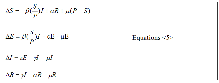
The rate equations for the SEIR model are shown in Equations <5> below:
The four states defined by the SEIR model by no means reflect the totality of compartmental models in epidemiology. In many cases, the population itself is segmented. The reproductive rate of a disease, the incubation rate, recovery rate, and mortality can all vary based on socio-economic factors, gender, age, and infrastructure (health care, sanitation, water quality). For many studies, the population itself is divided based on these or other factors that affect the transition rates from one state (compartment) to the next. For instance, studies involving finite birth and death rates may account for the maternal immunity conferred on new born infants; this transient immune state can be added to any of the models describe above. Models of sexually transmitted diseases (STDs) distinguish between males and females, partitioning an SI model into the states Sm, Sf, Im, If. Even more complex models include multi-serotype models for Flaviviridae viruses such as Dengue Fever. In Dengue Fever, previous infection by one strain of Dengue Fever can lead to more severe infection (and a greater viral load) in newly infected individuals. Multi-serotype models have been developed that account for historical infection in populations where several serotypes of the virus are circulating [5].
Limitations of Finite Difference Models
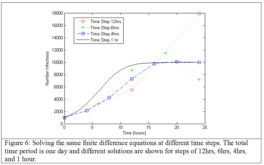
All of the equations used to define compartment models discussed above represent Finite Difference equations. In a Finite Difference equation, the time step is fixed (e.g., one day, one hour) and the value at the current time step is used to predict the value at the next time step. Computationally efficient, this approach is fast and lends itself to simple solutions. Unfortunately, it is also inaccurate. In reality, time is a continuous variable. Trying to predict the number of people that will be infectious one day from now based on the number infectious now will give a different answer than trying to predict the number of people infectious one hour from now, given the number infectious now, and repeating that calculation every hour. If the variables in the compartment model are changing slowly relative to the length of the fixed time step, then a finite difference algorithm will behave well. However, if the variables are changing rapidly, for instance, at the onset of an epidemic, finite difference algorithms can produce nonsensical results. A graphical example of the problem with a simple finite difference solution is shown in Figure 6.
Discrete vs Continuous Solution
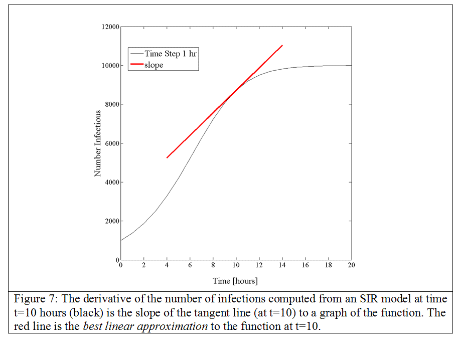
The figure shows four solutions to the exact same finite difference equation using time steps of varying length. Note that in this example the total population was 10,000 and the finite difference equations (for step sizes of 12 hours and 6 hours) actually predict an infectious population larger than the total population. This, of course, is impossible. One approach to solving this problem is to insist on a cutoff that prevents the algorithm from assigning solutions that are non-physical (i.e., values that exceed the total population or go negative). The sets of Equations 2, 3, and 5 are Finite Difference Equations. Difference equations are valid when the state variable can only assume discrete values. For example, a single coin is heads (1) or tails (0). However, as we discussed above, for a large enough system the Law of Large Numbers allows us to define continuous probabilities to the state variables. In a study of the rate of change in a function of continuously changing variables, the rate of change of the variables can be expressed by their derivatives. The finite difference equations then become differential equations. For a real valued function like time, as in equations 2, 3, and 5, the rate of change of the function or derivative at a particular time t is given by the slope of the tangent line to a graph of the function at that time, as shown in Figure 7. The value of the slope may be derived from a linear approximation to the function at that time.
Numerical Integration
Now consider the number of infections as a function of time from our finite difference approximation to an SI, SIR, or SEIR model. Each of the state variables is continuous function of time. For example, the total number of infections at time t is represented by:
I(t) = f(t) <equation 6>
Where summing the finite difference equations above provided an estimate to f(t) for various time steps. To estimate the slope of the tangent (or secant), m(t), for changes in I near time t, using a linear approximation to <equation 6> we can write:
This estimate of the slope gets better and better as δt gets smaller and smaller. Using the notation first introduced by Leibniz, in the limit δt→0 , we replace δt with dt and the slope of the function I(t) becomes its derivative dI(t)/dt given by:
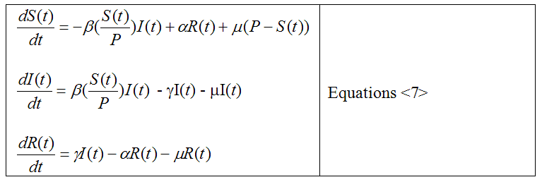
Whenever this limit is defined at some time, t, the function is differentiable at t and, therefore, continuous in time. Using our SIR model as an example, the corresponding differential equations are:
In all of these equations the time, t, is the only independent variable. S(t), I(t), and R(t) are all dependent variables (they depend on time). Differential equations with only one independent variable are called Ordinary Differential Equations (ODEs). Solving (integrating) these equations to get S(t), I(t) and R(t) is more complex than the computations we described above, but computational methods have been developed. ODEs can be solved numerically by performing the computation at various time step lengths and then picking a time step short enough to minimize the computational error below a selected threshold. An example of this approach is the Runge Kutta Fehlberg method that takes advantage of such an adaptive step size algorithm.
Nonlinear Models
The finite difference models are subject to several other assumptions and limitations. The first assumption is that the model parameters (e.g., β,ε,γ,α) are all constant in time. For some diseases such as the seasonal flu and many childhood disease, transmission rates are thought to vary seasonally, increasing when schools are in session and decreasing during the summer when the weather is warmer and schools are not in session (in the Northern Hemisphere). In some more advanced models, the constant β is replaced with a time varying function (typically modulated sinusoid ally with time). The bilinear interaction term,
is itself a simplification valid only when the probability a susceptible individual will become exposed by an infectious individual is independent of the number of other infectious individuals around. For some infectious diseases, the exposure process is thought to be nonlinear and dependent on the environmental viral load [6]. In such a nonlinear interaction, the immune system becomes swamped by repeated exposure to infectious individuals. More complex models that account for this effect been developed. The nonlinear response of the immune system can be described by a model where the infection probability increases nonlinearly as:
The Role of Noise
The finite difference solutions described above and the solution to a compartment model that uses ordinary differential equations (ODEs) can be done in either a deterministic or stochastic way. A deterministic solution can be thought of simply as an accurate or “exact” solution to the mathematic equation at hand. Numerical solutions (equations solved with a computer or spreadsheet) are subject to the numerical precision of a computer and often have round-off errors. Stochastic solutions introduce a deliberate level of random noise to the computation. Why would anyone ever want to add noise to a computation? It turns out that many dynamical processes in nature, because they are stochastic or naturally noisy, cannot be accurately modeled using deterministic equations. To understand the dynamics of an infectious disease, it is useful to look at the time varying trajectory of the disease in a Phase Space. J. Willard Gibbs first introduced this concept in 1901 [7].
If we think of a host population containing a circulating infectious disease as our “system”, then the Phase Space for this system is a space that represents every possible State of the system. If we model the system with, for example, and SIRS model, the variables that define the state of the system are S, I, and R. These variables are constrained by the relationship:
S(t)+I(t)+R(t) = Total Population (for all times t) <Equation 6>
For constant population we can divide each of the state variables, SIR, by the total population so they are normalized (have a range from zero to one). Every possible state of the system is then defined within a unit cube with Axes S, I, and R, each ranging from 0 to 1. As the State of the population changes, more people may become infectious, people may recover, etc. Over time, the set of points that represent the changing state of the system define a trajectory in this phase space.
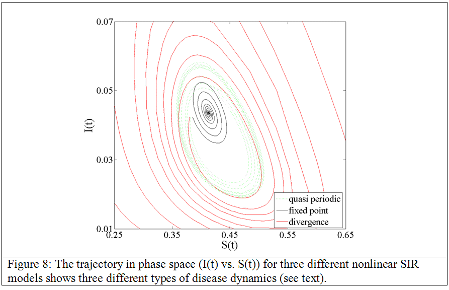
There are many possible trajectories for an infectious disease and studying them reveals something of the dynamics of the system as a whole. In general, a phase space can be of very high dimension (including many state variables) but often it is possible to learn about the dynamics by looking as a lower dimensional slice or cut through the complete phase space. For the compartment models discussed in this paper, the process of infection depends on a function of the variable S and I. Consider a phase space that plots the trajectory of a system in these two variables, I(t) vs. S(t). Three different examples trajectories are shown in Figure 8.
All three examples were generated with an SIR model using a nonlinear interaction term. The first trajectory (in black) shows a path that spirals in to a single fixed point. The trajectory leads to a single, final, point of endemic infection. Most deterministic bilinear SIR models will eventually evolve to such a fixed point.
The red trajectory represents an unstable dynamical state for an infectious disease. This trajectory is spiraling outward. The state variable S and I exhibit larger and larger oscillations. Eventually, the infectious population will spiral out to I(t) = 0 for some t an d disease becomes extinct. The red trajectory represents an unstable limit cycle. What is a stable limit cycle? Consider, for example, the seasonal flu. It comes and goes every winter in the Northern Hemisphere. If the flu were to occur on exactly the same date (or dates) every year, its trajectory would not only be stable, it would be perfectly periodic. As discussed above, some models of the seasonal flu include a periodic modulation to the transmission coefficient, turning the epidemic on and off with the seasons. A periodic trajectory would show up as a closed orbit or closed loop in phase space.
Exercise: In STEM, open the project explorer and run the custom Scenario for Cuba. Look at the time series and phase space plots. Observe the quasi-periodic orbit (Figure 8). Stop the Simulation and go to the designer perspective. In the project explorer open the Cuba project and expand the node labeled “decorators”. You will see under this mode the disease model used in the scenario. Double click on the Disease Model "Stochastic Flu" and follow the instructions to edit the model so you can change the disease parameters with the property editor. Try raising the immunity loss rate to 0.04. Rerun the simulation. What happens to the trajectory in phase space? Lower the rate to 0.03. Rerun the simulation. What happens to the trajectory in phase space?
Outbreaks of influenza occur virtually every year; both their magnitude and precise dates vary year to year. The seasonal flu is a quasi-periodic event. A deterministic computational model will never produce this type of dynamics. Figure 9, shows a example of a quasi-periodic trajectory (in green). The limit cycle is stable because the path will never collapse into a fixed point and it will never diverge to a point where I(t) = 0 (extinction). However, the orbit is not closed. This stable limit cycle will continue to oscillate around the same region of phase space but it will not come back on itself and it will never retrace a constant path. It is quasi-periodic. This trajectory was generated with a non-linear, stochastic model. The noise build into the stochastic simulation is like an excitation of the deterministic trajectory. A stochastic simulation which adds a small amount of noise to a proper solution to the differential equations defining a compartment model for an infectious disease allows the dynamical system to “explore” the phase space of possible trajectories. If the noise level is small, the system can enter stable limit cycles and follow either periodic or quasi-periodic trajectories. Stochastic models are often required to capture the true dynamics of infectious disease.
Transportation Models
Transportation Between Regions in Spatiotemporal Models
The models we have discussed so far represent the evolution of an infectious disease in time only. None of them represents the geographic distribution of people or how they move about in space. A compartment model that deals only with the trajectory of a disease in time implicitly assumes that the population (or populations) in question is so well mixed that there is no need to model the spatial distribution of people. However, for very large scale simulations, the details of population distribution, transportation, trade, even wild bird migration can all be important factors in understanding the evolution of an infectious disease in space and time. Please read the section on Transportation Models to see how the distribution, circulation, and migration of populations are implemented in STEM.
Built-in compartment models in STEM
STEM comes with a range of built-in textbook models for infectious disease.
DeterministicSIDiseaseModelImpl: A basic SI disease model that is deterministic (i.e. does not include random noise)
DeterministicSIRDiseaseModelImpl: A basic deterministic SIR disease model
DeterministicSEIRDiseaseModelImpl: A basic deterministic SEIR disease model
The following are implementations of disease models with random noise. The amplitude of the noise can be controlled using the gain parameter.
StochasticSIDiseaseModelImpl: An SI disease model that includes a noise component.
StochasticSIRDiseaseModelImpl: An SIR disease model that includes a noise component.
StochasticSEIRDiseaseModelImpl: SEIR disease model that includes a noise component.
Random noise does not reproduce the noise properties of making a random pick from a binomial distribution. The following are implementations of disease models pick from a Poisson distribution. These are "better" stochastic models but slower to compute. IMPORTANT: The Poisson disease models in STEM can only be used when the Scenario is using a Finite Difference solver.
StochasticPoissonSIDiseaseModelImpl: An SI disease model randomly infecting individuals using a Poisson distribution.
StochasticPoissonSIRDiseaseModelImpl: An SIR disease model randomly infecting individuals using a Poisson distribution
StochasticPoissonSEIRDiseaseModelImpl: An SEIR disease model randomly infecting individuals using a Poisson distribution
ForcingDiseaseModelImpl: An SIR disease model where the transmission rate varies using a sine function. The period of the fluctuations is controlled by the Modulation Period parameter, and it is possible to shift the peak(s) using the Modulation Phase Shift parameter. For this model, Transmission Rate is the scaling factor of the sine function, and the "Seasonal Modulation Floor" parameter determines the lower bound of the transmission rate. It is also possible to narrow or widen the seasonal duty cycle using the Seasonal Modulation Exponent parameter, the sine function exponent. You can add random noise to this disease model using the Gain parameter.
GaussianForcingDiseaseModelImpl: An SIR disease model where the transmission rate varies using a Gaussian function. The period of the fluctuations is controlled by the Modulation Period parameter, and it is possible to shift the peak(s) using the Modulation Phase Shift parameter. For this model, Transmission Rate is the scaling factor of the Gaussian, and the "Seasonal Modulation Floor" parameter determines the lower bound of the transmission rate. Sigma^2 is the variance. It is also possible to add noise to this disease model using the Gain parameter.
References
[1] R.M. Anderson, R.M. May, Infectious diseases of humans: dynamics and control, Oxford Science Publication, New York, 1991
[2] J Bernoulli (1713/2005) In: On the Law of Large Numbers, Part Four of Ars Conjectandi (English translation by O Sheynin), Berlin: NG Verlag, ISBN 3-938417-14-5
[3] J Bernoulli (1713) In: N Bernoulli, Ars Conjectandi, Opus Posthumum. Accedit Tractatus de seriebus infinitis, et epistola gallicé scripta de ludo pilae reticularis. Basel: Thurneysen Brothers. OCLC 7073795
[4] D Bernoulli (1766) Essai d’une nouvelle analyse de la mortalite causee par la petite verole. (An attempt at a new analysis of the mortality caused by smallpox and of the advantages of inoculation to prevent it). Originally published in Commentarii Academiae Scientiarum Imperialis Petropolitanae (V5). English translations L Sommer (1954 Jan) Econometrica 22:23-36; and S Blower (2004 Sep), Reviews in Medical Virology 14(5):275-288
[5] JW Forrester (1958) Industrial dynamics: a major breakthrough for decision makers. Harvard Business Review 36(4):37-66. http://www.bt.cdc.gov/agent/smallpox/overview/disease-facts.asp
[6] DA Cummings, RA Irizarry, TP Endy, A Nisalak, D Burke (2004) Traveling waves in dengue hemorrhagic fever incidence in Thailand. Nature 427:344-347
[7] W-M Liu, HW Hethcote, SA Levin (1987) Dynamical behavior of epidemiological models with nonlinear incidence rates. J Math Biol 25:359-380
[8] JW Gibbs (1902) Elementary Principles in Statistical Mechanics. New York: Scribner
For Further Reading
See a great wikipedia article on Compartment models in Epidemiology.


