Difference between revisions of "2019 novel Corona Virus Model"

Revision as of 14:06, 12 March 2020

STEM Contents Page

The 2019 novel Corona Virus (nCoV) Model is an all in one archive available on the download page that allows you to install and run a global model to study 2019-nCoV.

Please Observe: The precise epidemiological parameters are not known at this time. The downloadable scenario can be used to see how
changes to the parameters changes the spread. 

Additional documentation

relevant to installing and running the model

Please see the following wiki pages for help

1. Importing and Exporting Projects
2. using the The STEM UI and Map View
3. setting up Simulation Data Logging
4. Triggering interventions

Please observe: Logging the simulation data from a Global scenario to a delimited file takes an enormous amount of memory and should only be attempted when STEM is 
running on server (headless and with lots of  memory allocated to the heap). Please see: Running STEM Headless 
To test logging on a laptop please set up a smaller scenario with fewer countries. 
When logging on server please look at the buffer size setting in the logger object. You can adjust to buffer size to balance performance based on the memory available on your machine.

Getting the Downloadable Scenario

Please visit the downloads page and download the 2019 nCoV model.

Extract the archive to your local file system. It contains four primary components.

Archive and it's contents

All four of these components must be imported directly into your STEM work space (not nested in another folder). If you already have the GlobalGeography or the SuperContinentExamples projects installed you need not reinstall them (but they are required to run the scenario).

• The project ncov.eclipse.org.coronavirus is the model builder project containing the disease model.
• Project folder CoronaVirus contains the global scenario.

Setting up the model

Once you have installed all four projects and can see them all, un-nested, in the project explorer (in your workspace),

1. navigate to the ncov.eclipse.org.coronavirus
2. open the models folder.
3. make sure you are in the designer perspective
4. double click on coronavirus.metamodel
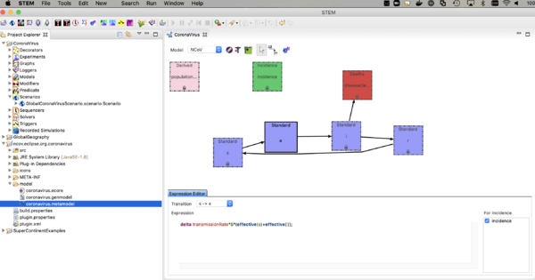
5. you should the see the compartment model itself as shown below.
6. After importing the scenarios you may also click the gear icon in the model builder to recompile all the generated Java code and plugins (this is only necessary on some systems, but it's a good idea to do once on import.

The nCoV model is an SAIR model where A represents individuals who are shedding virus (infectious) but asymptomatic. The I compartment represents individuals who are infectious and symptomatic. The incidence (or transition from S -> A, depends on the sum of the fraction infectious in both A and I. Click on the transition and see the expression in the expression editor. You can watch the youtube video on the model builder to see how this works.

The model looks a lot like an SEIR model but there is no incubation state (E) or incubation rate (you could add that if you want to). The reason to explicitly model the A compartment is that one can add interventions (predicates, modifiers, and triggers) based on the I state but not A. The rate individuals move from A -> I is called the "Symptom Appearance Rate" in this model. Next,

• Navigate to the CoronaVirus project,
• open the decorators folder,
• and double click on the disease model (not the infector) to open it in the resource window. The disease model is a little black icon with a caduceus (the symbol of medicine). The infector is the same symbol with a capital letter 'I' in one corner.
• Click on it in that window and open the property view below.

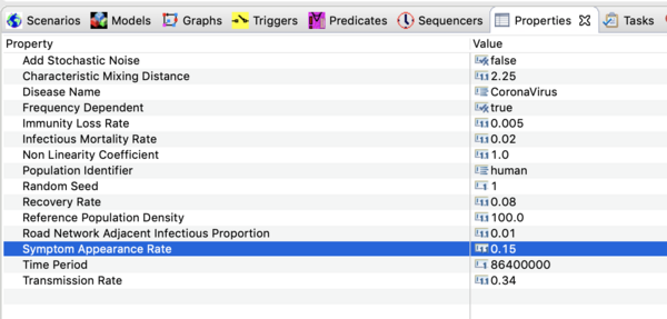
You should see all the parameter values defined in this model as shown in the image below.

Precise values are not known at this time. The settings used in the downloadable scenario are based on upper estimates for the basic reproductive number reported in the literature as of Jan 30, 2020. R_o depends on the transmission rate, β , the recovery rate, γ , and the infectious mortality rate, μ .

Ro = β/[γ + μ]

With the values shown above this puts R_o ~ 3.4. The first case appeared in mid December 2019. If you run the simulation for 45 days you will see the current settings over estimate cases in China but under estimate incidence from air travel. The high end estimate for R_o is likely too high and the build in STEM air travel model probably underestimates recent traffic.

Running the model (for the first time)

Before you try to run the model, navigate to the command bar ....

• On a mac go to >STEM>Preferences>STEM>Simulation Management one windows >Windows>Preferences>STEM>Simulation Management
• un-check scenario caching
• set the time delay to about 150 msec

Then navigate to

• Preferences>STEM>Solver
• and increase worker threads if you workstation has more than two core (for example 4 threads will help performance).

Remember you are about to load a global simulation.

• Open the Scenarios folder
• Select the GlobalCoronaVirusScenario.scenario Scenario.
• Right click and click STEP the little foot step icon. (please do not click run yet)
• Depending on your laptop you might want to get a cup of coffee. The model has been tested on a 2018 macbook pro and the global graph does load without error, but it will take a couple of minutes to load.

Once the map loads you can pan by clicking and draging the map and zoom with up and down arrows.

• Right click on the ocean and select a gain factor of 1,000,000
• Step a few more times until you are at about day 4
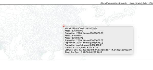
• Zoom in on China until you can find the red administrative zone where the infector seeded the first case(s). This is Wuhan Shiqu (Wuhan City).
• Double click on Wuhan to start a time series monitor for that region.

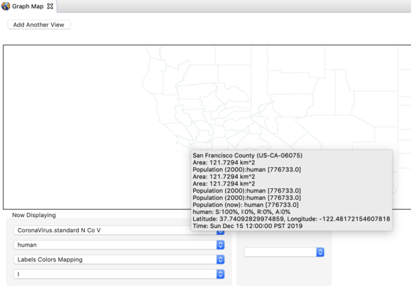
• Zoom and Pan until you find San Francisco in California, and double click to set up a monitor for that region.

• Right click on the map again and set the gain factor down to 1000. This is high enough to see the early cases.
• Click "run"
• When you get to about 50 days (Sequencer time Jan. 30) you might hit pause and then step again until you see evidence for infection via air travel.
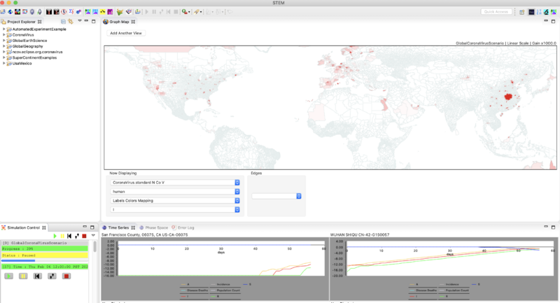
• At 57 days (Sequencer time Feb. 6) the simulation should look like this. Note that in the image below both time series monitors have been set to show a logarithmic scale (right click on the monitor to do that).

Next Steps

• Once you have the scenario running, go back to the property view for the disease model and see how changing the parameters effects the spread.
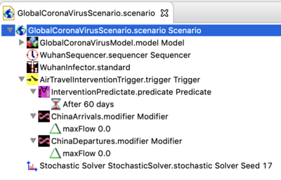
• As of Jan 31,2020 an example intervention has been added to the downloadable scenario. The new Scenario structure is shown below.

• In this example, the predicate is set to trigger the intervention at 60 days (so it does not change the behaviors described above). At 60 days, the edges regulating air travel two or from China are modified to set the max flow to zero for international travel. You can change this by changing the time parameter in the modifier. Please see the interventions documentation to learn about Triggering interventions in general.

Acknowledgements

The STEM community would like to acknowledge Dr. Brian M. Gurbaxani(CDC/DDPHSS/OS/OTI) for suggesting the structure of this model.