Notice: this Wiki will be going read only early in 2024 and edits will no longer be possible. Please see: https://gitlab.eclipse.org/eclipsefdn/helpdesk/-/wikis/Wiki-shutdown-plan for the plan.
Difference between revisions of "STEM Disease Models"
(→Mosquito Population Model) |
(→Models of Population) |
||
| (36 intermediate revisions by 4 users not shown) | |||
| Line 1: | Line 1: | ||
[[Image:STEM TOP BAR.gif|800px]] | [[Image:STEM TOP BAR.gif|800px]] | ||
| − | {| align=" | + | {| align="right" |
| __TOC__ | | __TOC__ | ||
|} | |} | ||
| Line 27: | Line 27: | ||
== MacDonald Ross Disease Model == | == MacDonald Ross Disease Model == | ||
| − | + | ||
| + | Our model for malaria transmission is based on work originally carried out by Ross (1911) and MacDonald (1957). Details can be retrieved from [[MacDonald Ross Disease Model|'''individual page for MacDonald Ross Model''']]. | ||
| + | |||
| + | == Full Dengue Disease Transmission Model == | ||
| + | |||
| + | We created a so called "full model" in order to capture a comprehensive picture of dengue transmission between host (human) and vector (mosquito) populations in STEM. Details can be obtained on the [[Dengue Disease Transmission Model| '''introductory page of dengue model''']]. | ||
| + | |||
| + | == Polio Disease Transmission Model == | ||
| + | |||
| + | This model mainly focuses on capturing wild poliovirus transmission and modeling the risks of circulating vaccine-derived polioviruses (cVDPVs) from OPV using nine compartments. Details can be obtained on the [[Polio Disease Transmission Model| '''introductory page of polio model''']]. | ||
== Nonlinear Models == | == Nonlinear Models == | ||
| Line 69: | Line 78: | ||
= Models of Population = | = Models of Population = | ||
| − | + | STEM also allows users to model populations (human, insect, animimal, etc). Please see the page on [[STEM Population Models]] for detailed information on the may types of population models available | |
| − | + | ||
| − | + | ||
| − | + | ||
| − | + | ||
| − | + | ||
| − | + | ||
| − | + | ||
| − | + | ||
| − | + | ||
| − | + | ||
| − | + | ||
| − | + | ||
| − | + | ||
| − | + | ||
| − | + | ||
| − | + | ||
| − | + | ||
| − | + | ||
| − | + | ||
| − | + | ||
| − | + | ||
| − | + | ||
| − | + | ||
| − | + | ||
| − | + | ||
| − | + | ||
| − | + | ||
| − | + | ||
| − | + | ||
| − | + | ||
Revision as of 13:09, 13 April 2012

New models are continually being added to STEM. Today STEM comes with a variety of basic models which implement algorithms such as those found in RM Anderson & RM May's textbook on Infectious Diseases of Humans: Dynamics and Control, Oxford and New York: Oxford University Press, 1991. ISBN 0198545991. STEM also includes more advanced models created by groups investigating current problems in epidemiology. As a framework users are also encouraged to create their own models and to even contribute them back to STEM.
Basic Models
STEM comes with implementations of many standard epidemiological compartment models. These include both Stochastic and Deterministic SI, SIR, and SEIR models as well as models with seasonal forcing and nonlinear interaction terms.
SI and SIS models
The simple two-state SI or SI(S) model is useful in describing some classes of microparasitic infections to which individuals never acquire a long lasting immunity. Certain RNA viruses such as rhinoviruses and coronaviruses (the common cold) mutate so rapidly that individuals recently recovered from a cold will still be susceptible to other strains of the same virus circulating in a population. In a simple model for this process, individuals never enter a recovered state, but rather alternate between being susceptible and being infectious.
SIR and SIRS models
More generally, after exposure to microparasitic infection, individuals who recover from a disease will enter a third state where they are immune to subsequent infection. This Recovered State, R, appears in the SIR(S) compartment models. For infections that confer lifelong immunity in the recovered state, an SIR model is appropriate. Typical examples for which an SIR model is used include Paramyxovirus (measles) and Viral Parotitis (mumps). In cases involving the Orthomyxoviridae viruses (which cause seasonal flu), immunity is not lifelong and may decrease over time. Immunity loss can reflect a decrease in an individual’s immune response, or a genetic drift in the circulating strain of virus that diminishes the effectiveness of the acquired immunity. In either case, an SIRS model represents the rate at which people in a Recovered state return to a susceptible state.
SEIR and SEIRS models
Some infectious diseases are also characterized by an incubation period between exposure to the pathogen and the development of clinical symptoms. If the exposed individual is not infectious during this incubation period (e.g., not shedding virus), it is important to model the incubation time explicitly. Note that there is a difference between an incubation time and a period of latency. A virus may or may not be dormant when an individual is in an exposed state. It is important to model the exposed (E) state explicitly when there is a delay between the time at which an individual is infected and the time at which that individual becomes infectious. In this case an SEIR(S) model is appropriate. Smallpox, for example, has an incubation period of 7-14 days
The disease models in STEM are implementations of these compartment models expressed as differential equations. These differential equations have a variety of parameters that are similar to the constants in a chemical rate equation. Users can easily change the basic parameters of any model in STEM with a text editor (called the property editor). This tunes the model based on the particular disease of interest. New models with even more advanced mathematics can easily be added to STEM - but that does take some knowledge of the Java programming language and of Eclipse. Please see the Tutorials and User Guides for detailed information on how to do this.
Once you have put together a model with a geographic region and other data (like transportation, time, and human population) you can easily export your work and share it with other users of STEM. In this way STEM is intended to promote scientific collaboration allowing researchers to build on each others work. See the section on Importing and Exporting Projects for instructions on how to do this and for information on some example scenarios.
Advanced Models
MacDonald Ross Disease Model
Our model for malaria transmission is based on work originally carried out by Ross (1911) and MacDonald (1957). Details can be retrieved from individual page for MacDonald Ross Model.
Full Dengue Disease Transmission Model
We created a so called "full model" in order to capture a comprehensive picture of dengue transmission between host (human) and vector (mosquito) populations in STEM. Details can be obtained on the introductory page of dengue model.
Polio Disease Transmission Model
This model mainly focuses on capturing wild poliovirus transmission and modeling the risks of circulating vaccine-derived polioviruses (cVDPVs) from OPV using nine compartments. Details can be obtained on the introductory page of polio model.
Nonlinear Models
STEM also implements nonlinear versions of the basic compartment models where the bilinear transmission kinetics term (bSI) is replaced with a modle of nonlinear transmission (e.g., bSIν, ν > 1 (see Liu, W-M., Hethcote, H. W. and S. A. Levin. 1987. Dynamical behavior of epidemiological models with nonlinear incidence rates. J. Math. Biol. 25: 359-380). Nonlinear models can be used to model saturation or " swamping " of the immune system as a function of disease burden or repeated exposure.
Seasonal Tranmission (Forcing Function) Models
Sinusoidal Model
Many diseases exhibit periodic or quasi-periodic epidemics, the most well being seasonal influenza. Recent experiments using guinea pigs suggest that seasonal variations in influenza incidence may be explained by small changes in transmission rate due to changes in temperature and relative humidity (Lowen et al., 2007; Shaman et al., 2009). Since SIR(S) disease models have an intrinsic tendency to oscillate (although with dampened effect), such changes can be further amplified by dynamic resonance caused by the population dynamics of the host-pathogen system (Dushoff et al., 2004).
As defined by Dushoff (2004), a SIR(S) model has a natural frequency

where γ is the recovery rate, α the immunity loss rate, and Ro the basic reproductive number. While a deterministic SIR(S) model with constant transmission will not exhibit sustained oscillations, it can demonstrate “damped” oscillations at this natural frequency, with the epidemic eventually dying out or tending to a fixed point of endemic infection. If the transmission rate includes a periodic excitation term (a forcing function) tuned to the same resonant frequency, seasonal oscillations may be sustained. If the frequencies differ, as is the case for any forced harmonic oscillator, the system may exhibit sustained oscillations with “beats” resulting in some epidemics that are larger than others.
STEM includes advanced models seasonally modulated transmission coefficient β(t). A deterministic SIR(S) model with constant transmission will never produce sustained periodic epidemics or seasonality (Dushoff et al., 2004). The simplest seasonal transmission function implemented in STEM uses periodic forcing function:
β(t) = βo[(1 - x) + x sin(ωt + φ)]
where βo is the(max) transmission amplitude and x determines the periodic part of the excitation function (0<=x<=1).
Gaussian Model
We are also developing a periodic excitation function based on a linear combination of (periodic) gaussian excitations. This function may be useful in modeling data where the size of the epidemic varies year to year based on known differences in transmissibility of a disease (for example variations in the dominant serotype or strain).
We define β(t) as:

where i is the index of the yearly influenza season; βi is the peak transmission coefficient for season i; (1-ρi) is the fraction by which transmission varies seasonally in season i (0 < ρi < 1.0); ti is the day of peak transmission for season i; g(x, σi) is the probability distribution function of a Gaussian distribution with mean 0 and standard deviation σi; and ξ(t,ti) is the mixing function. The day of peak transmission, ti, is defined so that the transmission function has a period of exactly 1 year, with constant phase, φ. That is transmission peaks φ days after January 1 of season i. The joining function, ξ(t,ti), smoothly joins adjacent Gaussians so that β(t) is only dependent upon a single Gaussian during the period of season i where most transmission occurs
Interpolation of Sampling Points
The seasonal variations of the incidence of a disease can be caused by different things. Climate changes can be the reason as mentioned above, but even the beginning and the end of the school year can have an influence on the disease. In order to be able to model all kinds of seasonal variations, the STEM user should be able to specify every possible excitation function, which can be done as shown in the following. The user specifies the transmission rate for several days in the year and interpolation is used to compute the transmission rate for all remaining days. The simplest interpolation method is linear interpolation. To get a smooth function spline interpolation can be used.
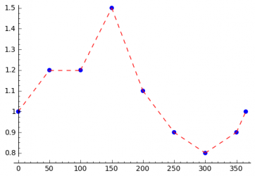
Linear Interpolation
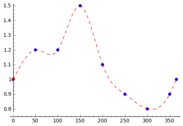
Spline Interpolation


Models of Population
STEM also allows users to model populations (human, insect, animimal, etc). Please see the page on STEM Population Models for detailed information on the may types of population models available