Notice: This Wiki is now read only and edits are no longer possible. Please see: https://gitlab.eclipse.org/eclipsefdn/helpdesk/-/wikis/Wiki-shutdown-plan for the plan.
Running an Automated Experiment
Overview
The STEM AI plugin is provide a function called Automatic Experiments. The plugin uses a Nelder-Meade downhill simplex algorithms to automatically optimize any disease model with respect to reference data. The error function use (defined in the class SimpleErrorFunctionImpl.java) computes the normalized root mean squared error (nrmse) with respect to reference and predicted daily incidence. Daily incidence is the quantity reported by public health. The error in daily incidence defines the surface that the algorithm "walks down" given the user define parameter space. As of STEM 4.0.0 users may also select a ComplexErrorFunction to optimize their models with respect to daily incidence, cumulative incidence, and/or cumulative deaths or even a combination of all three.
Running an Experiment
If you're trying to fit the output of a disease model to a reference, for instance to actual incidence data collected by public health surveillance, manually determining the parameter values for a good fit can be very time consuming and often impossible. That's where the Automatic Experiment feature in STEM comes in handy.
First, to familiarize yourself with automatic experiments in STEM, download the sample project available here:
http://www.eclipse.org/stem/download_sample.php?file=AutomatedExperimentExample.zip
and also read the documentation for this example here:
http://wiki.eclipse.org/Sample_Projects_available_for_Download#Automated_Experiment_Example
An automatic experiment will run a sequence of STEM simulations, each time varying parameters of the model and compare to a reference. It tries to minimize a error function, calculated by comparing the output (simulation log) to the data in a reference folder (where data is stored in the same format as for STEM log files). It walks the parameters of the model until it is unable to improve upon the calculated error beyond a specified tolerance. At that point the automated experiment either halts, and the optimal set of parameters found can be retrieved from the "Current Values" view on in the Automatic Experiment STEM perspective, or it restarts itself using an initial set of parameter values matching the best parameter values found so far. If the automatic experiment converges to the same set of parameter values (and error) a second time, the automatic experiment is done.
When an automatic experiment is started, STEM automatically switches to the Automatic Experiment Perspective.
This perspective has a view with five tabs:
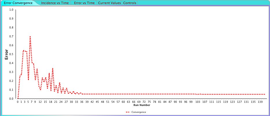
1. Error Convergence. Shows a plot where the X axis is the simulation number (starting from 0) and the Y axis is the calculated error. When running the automatic experiment you'll see how the error converges towards a smaller and smaller value. if your automatic experiment is configured to restart itself after convergence, you can see the when this happens in the plot since the error suddenly becomes large again.
2. Incidence vs Time. Shows you the incidence (new cases in a given time period) calculated by your model versus the incidence in the reference data. This plot is especially useful since the only error function currently implemented compares incidence only.
3. Error vs Time Shows the error between the reference data and the current model output for each time step of a simulation. It also shows the error for the best set of parameter values found so far.
4. Current Values. The top row in the table on this page shows the best set of parameters discovered so far, as well as the associated error. The rest of the rows shows a history of the 10 last set of parameter values and the bottom row is the values used in the current simulation.
5. Controls. In the Controls tab you can stop the currently running automatic experiment, or you can restart it using any set of parameter values you specify.
Create an Experiment and Choose an Error Function
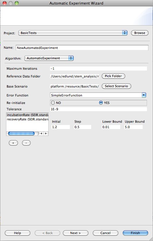
To create a new automated experiment in STEM, click the "New Automatic experiment" toolbar icon. A new wizard shows up similar to the one in the figure below.
Simple Error Function (default)
First, specify a name for your new automated experiment. You can give it any name you want. Next, pick the algorithm to use. Currently there is only one option available, "AutomaticExperiment" which is an implementation of a Nelder Mead downhill simplex numerical optimization algorithm. See this [page] for a description of this algorithm.
The Nelder Mead algorithm can be configured as follows:
1. Maximum Iterations. If this number of simulations has ran without convergence to an error variation smaller than the tolerance, the algorithm stops or restarts itself (depending upon the setting of Re-initialize parameter see below). If you set it to -1, the algorithm will run until the error converges (-1 essentially means no maximum number of iterations)
2. Reference data folder. This is the directory containing the reference data. The directory must contain the same files that STEM generates in its log output folders, e.g. an I_2.csv, Incidence_2.csv, S_2.csv etc. The current error function only requires the Incidence file. If the reference files are located in a folder inside the current project, the location is specified in a platform neutral manner and the project and associated automatic experiment can be shared with others.
3. Base Scenario. Clicking the "Select Scenario" button will allow you to pick any Scenario that is inside your current project. The base scenario the is the scenario the automatic experiment will run and compare to the reference.
PLEASE OBSERVE: In order to use Automated Experiments, the Base Scenario must include an integration solver like Runge Ketta Cash-Karp. Please see the STEM page on STEM Solvers
4. Error Function. The error function to use when comparing model output to the reference. Currently only a single error function "SimpleErrorFunction" is provided. It calculates a Normalized Mean Square Error (NMSE) between the incidence outputted by the model and the incidence in the reference data. NMSE is defined as follows:
where Is is the predicted incidence by the simulation and Ir is obtained from the historic reference data. We calculate the NRMSE as the root mean squared error over all time normalized by the difference between the maximum and minimum observed aggregated incidence. L is the set of all locations common to both the simulation output and the reference, and T is the set of all times for which we have observations.
5. Re-initialize. If this is set to Yes, the automatic experiment will restart itself using the current best (smallest error) set of parameter values found. The automatic experiment will stop of it converges towards the same minimal error twice in a row. If set to No, the automatic experiment will stop once it's converged to an error variation smaller than the tolerance.
6. Tolerance. The error tolerance determining when the Nelder Mead algorithm stops. If the error variation between multiple simulations is smaller than this tolerance, the Nelder Mead algorithm either stops or restarts itself. The smaller you make the tolerance the more simulations are needed for convergence, but the resulting set of parameter values becomes more accurate.
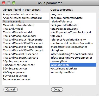
In the window in the bottom left you can add one or more parameter that you want to optimize in the automatic experiment. If you click the + button below the window, a dialog shows up displaying on the left all objects inside your current project that has parameters you can optimize.
The objects includes Disease Models, Infectors and Inoculators. If you select any object on the left, a list of the object parameters are shown on the right. If you select one of them and click Okay, it will show up ion the bottom left window and will be added to the set of parameters varied by the Nedler Mead algorithm. If you select the parameter in the window, you can specify the initial value for the parameter on the bottom right. You can also specify an initial step size and a maximum and minim value for the parameter used by the optimizer.
You can add as many parameters are you want to the automatic experiment, but the more parameters you have the larger the parameter space and the longer it might take for the algorithm to converge.
Often convergence to a global minima can be reached quicker by manually restarting the automated experiment on the Controls tab. If it seems that the error variation is small, restart the algorithm again using the best set of parameters. This can often speed things up compared to waiting for convergence below the tolerance.
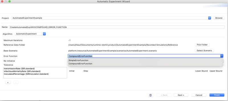
Selecting a Compound Error Function
When you create a new experiment with the Wizard (as shown above), you may chose to select the compound error function instead of the default. This allows...
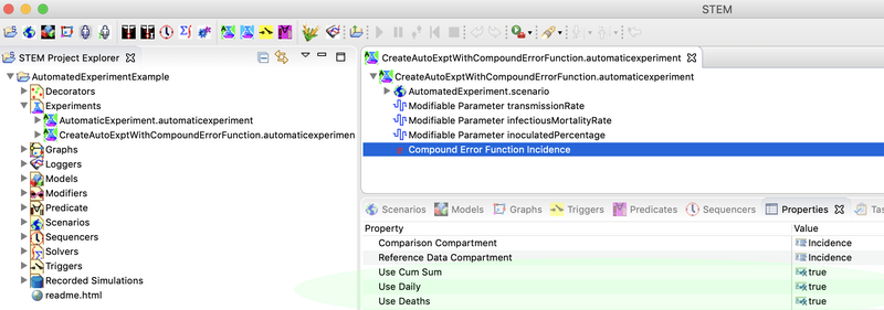
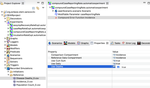
Configuring the compound error function is straight forward. Don't worry about this step when you first create it with the wizard. After you have created the automated experiment, open the Experiments folder in the project explored, double click on it to open it in the Resource Set view. Then expand it. Under the parameters you selected to define the optimization space, you will see a red letter "e". Click on the "e" and you will see the configurable options for the compound error function. You can pick any combination of daily incidence, cumulative incidence, of (cumulative) disease deaths simply by toggling the true/false selection to the right of each category. At least one of these properties must be true.
To run an experiment using the compound error function you MUST provide all three reference files as shown below. There are the population data for the regions being optimized, the daily incidence (cumulative is computed for you from this), and the cumulative disease deaths.
Please observe: The reference files must be named precisely as shown with a trailing integer indicating the highest administrative level for the data
in your reference and your scenario (_LVL). Please see the discussion above for the format of the files. The format is the same as that generated by
a STEM csv logger.
Running an Example Compound Error Function
An example experiment with a compound error function may be found in the second Sars-CoV-2 downloadable scenario (the one with the SEAIR project). The project contains two example Automated Experiments, the caseRepRateExpt.automaticexperiment that uses a simple error function and the compoundCaseReportingRate.automaticexperiment the uses a compound error function. You can download the scenario here.
downloadable scenario with an example compound error function


