Sample Projects available for Download

Sample Projects Available For Download

The STEM home page ([[1]]) contains several example projects users can import and run with STEM. STEM is designed to allow collaboration and sharing of work by simply importing and exporting projects from your workspace. For information on how to import a project please see: Importing and Exporting Projects

The Automated Experiment Example requires a STEM build from Sept 2, 2010 or later

The Multi-population Example requires a STEM build from Aug 31, 2010 or later

The Square Lattice demo described below requires STEM version dated July 1, 2010 or later

The SuperContinentExample project requires GlobalGeography to exist in the STEM workspace before it any of the examples can run.

Some of the example projects you can download are very large as they contain continents or even groups of continents. Before you try to run any of these large scenarios you must make sure you allocate enough system memory for STEM. If you don't do this the application may hang or crash with a "Heap Space" error. To allocate enough memory in Windows, create a shortcut for launching STEM. You may place this anywhere (e.g., on your desktop or on the quicklaunch bar).

Right click on the shortcut. Select "Properties" You should see a field in the Properties Dialogue labeled Target: to the right in the text field you will see something like

C:\stem_builds\stem\STEM.exe -vmargs -Xms812M -Xmx812M

To launch STEM with more memory you must add "virtual machine arguments" to the target line. For example, Target:

C:\stem_builds\stem\STEM.exe -vmargs -Xms896M -Xmx896M

Should work for the demo projects available.

On MAC OS X, using the finder, navigate to where the STEM application is located, right click and select "Show Package Content". Navigate to Contents->MacOS and open the STEM.ini file in an editor. Change the -Xms and the -Xmx lines to increase the memory, e.g. -Xms896M -Xmx 896M or more depending on how much memory is available.

Mosquito Density Model

This downloadable scenario demonstrates how the earth science data can be used to generate seasonal mosquito density estimates in Asia. The scenario (configured for Asia) requires the Global Geography Models and the Global Earth Science Models.

Automated Experiment Example

In this example, we have been given historical incidence data for a disease with unknown epi parameters and we want to try and determine what those parameters are. All we know is that the first cases showed up in Stockholm. If you import the demo project into your workspace, the reference incidence data is located under the "Recorded Simulations/Reference" folder in the Incidence_1.csv file (the other files in the folders are not used in this example).

We decide to try and fit an SIR model to the incidence data, and we would like to determine three unknown parameters:

1. What was the transmission rate of the outbreak?

2. How long were infected individuals shedding viruses (i.e. recovery rate)?

Given these two parameters it's possible to determine the reproductive number of the disease, an important epi parameter.

We also have one more unknown we would like to estimate

3. What was the initial background immunity to the disease.

Next, open the "Experiments" folder in the project explorer and double click "AutomatedExperiment.autmaticexperiment" it to bring up its editor. Select the top node in the editor and look at its properties in the properties view.

Automatic Experiment Editor

You will notice that the automatic experiment will run a scenario called "AutomatedExperiment.scenario". This is a basic SIR scenario where with a few initial cases of the disease occuring in Stockholm, as well as an inoculator to initialize the background herd immunity. You will also see that the algorithm being used to fit parameters to the reference is called "Nelder-Mead", and that an error function called "Simple error function" is used. Nelder-Mead is a well-known numerical model optimization algorithm, and the "Simple error function" calculates a normalized root mean square error between the incidence reported in the reference and the incidence calculated by the model simulation. The incidence is aggregated over all locations that are common between the model and the reference.

You'll also see that the maximum number of iterations is 1000. This means that at most 1000 simulations are run before either the algorithm stops or it restarts itself using the optimal set of parameter values found so far. If "Reinit" is false, the algorithm stops after either a solution having an error tolerance smaller than the one specified (1E-6) is found, or the maximum number of iterations is reached. If "Reinit" is true, the algorithm restarts itself again and stops only when the the solution converges towards the same minimum twice.

If you expand the top node "AutomatedExperiment.autmaticexperiment" in the editor you'll see that the automated experiment has 3 parameters it attempts to fit:

1. transmissionRate. The initial guess is 0.8 and the algorithm will use a step size of 0.2 when walking the parameter space for this parameter. Also, the maximum and minimim values for this parameter is 0.001 and 10. You can modify any of these values in the properties view.

2. recoveryRate. The initial guess is 0.2, step is 0.3 and the parameter value is between [0.001, 2.0]

3. inoculatedPercentage. The initial guess is 20, the step is 30 and the parameter is between [0,100]

All three parameters also reference the model the parameter belong to, in this case the first two reference the disease model and the last reference the inoculator.

To start running the automated experiment, right click on the "AutomatedExperiment.autmaticexperiment" file in the project explorer and select Run. STEM will automatically switch to the Automated Experiment perspective and the Automated Experiment view.

You'll see a view with tab options on top ("Error Convergence", "Incidence vs Time" etc.). Select "Current Values". You'll be shown a scrolling list of parameter values and to the right you'll see the calculated normalized root mean square error for that set of parameters.

The history of parameter values and the associated error is shown in the Current Values view.

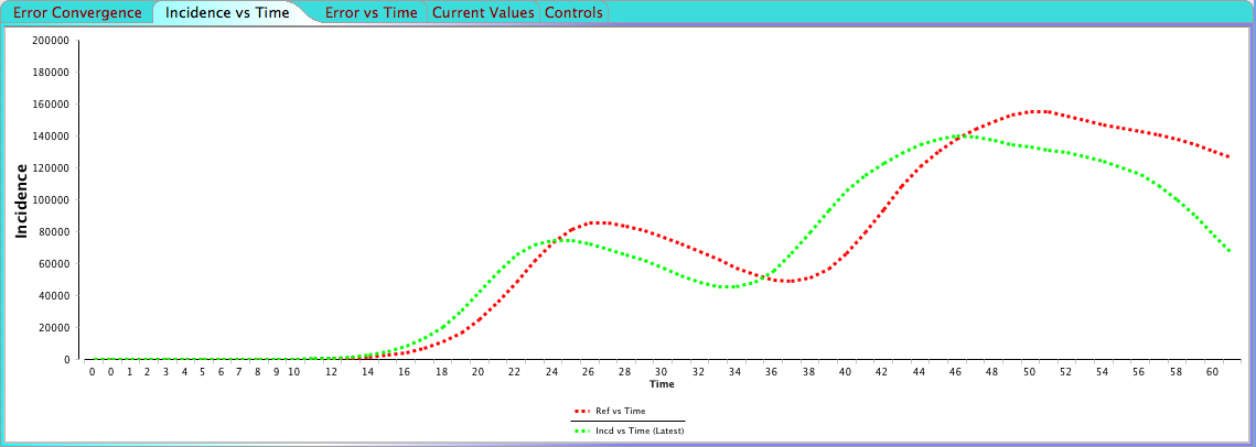
The "Error Convergence" shows a graph of the calculated error for each simulation and you'll notice how the error gets smaller and smaller. "Incidence vs Time" shows the latest incidence calculated by the current set of parameters compared to the reference incidence. Click the link below to see an animation demonstrating how the incidence is converging towards the reference.

The current calculated incidence versus the reference incidence Click here to see animation

"Error vs Time" shows the difference in incidence between the reference and the current model, compared to the difference in the best fit found so far. Finally, you can stop and restart an automated experiment using the "Contols" tab. When it looks like the algorithm has converged and the error is not changing much it is often useful to stop the experiment and restart it manually using the current optimal set of parameter values found. You can also specify any other parameter values on the Controls page and restart the experiment from those.

If you let the algorithm run until it completes (after about 2,200 simulations), it ends up with the following estimates for the parameters:

• transmissionRate: 1.192
• recoveryRate: 0.280
• inoculatedPercentage: 35.78.

You've probably already guessed it, but the reference data in this case was actually generated using a model with known parameter values. The values were 1.2 for transmission rate, 0.3 for recovery rate and the inoculated percentage was 35% (you can try plugging these values into the automated experiment, the error returned should be 0). You can force the algorithm to search for an even better fit by lowering the Tolerance parameter in the automated experiment (the tradeoff being that it takes longer to finish).

Each combination of parameter value tried and the resulting error is stored in a file called resultLog.csv in a folder AutoExpTempDir in the STEM workspace.

Multi-Population Example

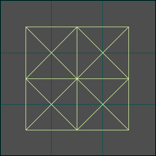
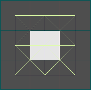
Figure 1a-b. Square lattice world where the anopheles and human population is evenly distributed on each lattice square (a), and where there is a human village located in the center square (b). The edges are the common borders where both anopheles mosquitos and humans are mixing.

The Multi-Population example contains two scenarios of very much simplified Malaria models spreading across a 3x3 square lattice world. In the first example (Figure 1a), each node contains the same number of humans (50) and the same number of anopheles mosquitos (10,000). In the second example (Figure 1b), there is a village in the center square lattice containing 1,000 humans.

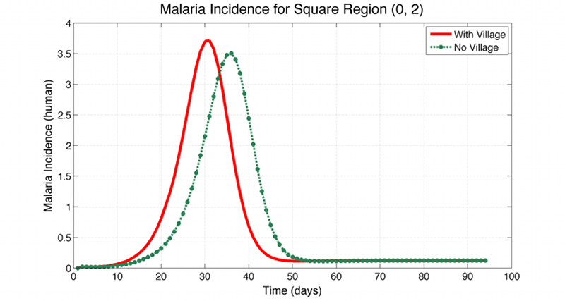
The disease is only spreading from infected humans to susceptible mosquitos or from infected mosquitos to susceptible humans, and it starts off by infecting 5 anopheles mosquitos in the upper left square. No infections transmit directly from human to human or mosquito to mosquito. The example also contains the log files from both scenarios, and a comparison between the incidence in the lower right square for both scenarios is shown in Figure 1c below. As can be seen, with the village in place, the incidence peaks about a week earlier for the lower right square. It should be noted, that in this simple sample model the mixing between anopheles members in two neighbouring nodes is at the same rate as the mixing between the human members of the very same nodes. In a real world example one would have to specify these rates seperately.

Figure 1c. Comparison of the daily incidence for both scenarios available in the Multi-Population example. In the scenario having a village in the center square, the incidence in the lower right square peaks about a week earlier than without the village.

Square Lattice Example

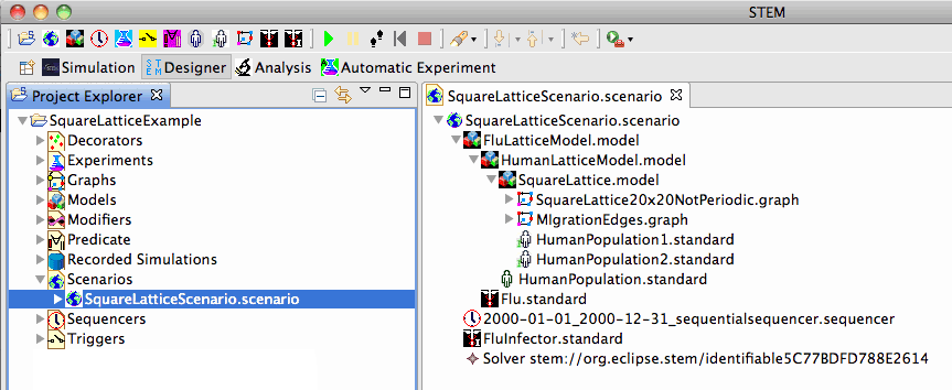
Figure 2. Square Lattice Example

The Square Lattice Example shows how a square lattice, migration edges, and initial population gradient can be used to model the interaction between an infected and uninfected population. It also demonstrates the hierarchy required to set up a SquareLatticeScenario.scenario: disease models must contain population models, and population models must contain initialized graphs, etc.

As illustrated in the figures that follow, the Square Lattice Example shows how to use migration edges to create two population gradients that cause a population to spread out over space and time. Only one of two populations is initially infected with a disease so you can see both the spread of disease within the original population as well as the eventual transmission from the infected population to the susceptible group when they meet. To accomplish this, the example uses both a standard population model and a Population Initializer (see Figure 1 below and the Tutorial on Using Structured Populations). The population initializer places an initial number of individuals at two separate locations at time zero. Migration edges exist (with equal migration rates) in both directions between all sites but, because there is a population gradient, the population spreads out or diffuses across the lattice.

Note that the components that appear when you click on SquareLatticeScenario.scenario (Figure 2, right) are hierarchical. The two population initializers are placed within the innermost option, HumanPopulation1.standard. The standard population object (HumanPopulation.standard) depends on the existence of the initialized graph and, therefore, is placed in the outer HumanPopulationModel. Both of these submodels are components or bundles that can be reused across many scenarios. Finally, the disease itself (Flu.standard) is a human disease that depends on a contained human model so it is placed in the outermost model of the hierarchy (FluLatticeModel). This too is a reusable component.

The Infector for the disease (FluInfector.standard) depends on a model of what is already known about the disease. An infector changes the state of a model by moving individuals from the susceptible state to the infectious state (given the presence of the indicated disease). As such, an infector is really part of the scenario - the topmost level in the hierarchy that contains ALL models.

In the figures below, you can see the initial population spread by migration edges. In the same simulation at runtime you can select the disease as the property to display and watch the disease spread.

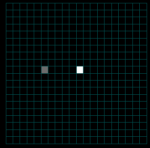
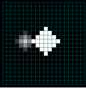
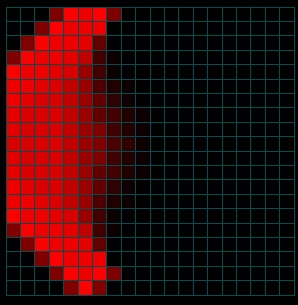
Figures 3a-c. Spread of the Human Population by Migration Edges

The figures above show the spread of the population itself by migration edges. The population is seeded in the center (10x10) and in a node just left of center. The center population is much larger than the smaller seed to the left (the intensity is saturated). Only the population to the left is infected initially. Open the infector and the population initializer in the property editor to see the initial values. As the infected population on the left spreads, it eventually makes contact with and infects the main population spreading from the center.

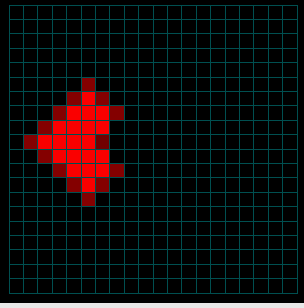
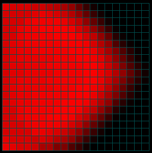
Figures 4a-c. Spread of the Disease

The figures above show the same simulation but display the fraction of people infected as a function of time. Note that the intensity does not reflect the NUMBER of infections (only the fraction). When the infected population on the left reaches the much larger fully susceptible (but not yet infected) population spreading from the right, the intensity actually goes down as the fraction of people infected drops (initially) at the point of contact (see the middle image above). Eventually (right) the main population also becomes infected.

Mexico/USA H1N1 Scenario

The Mexico/USA H1N1 Scenario was created in the early spring of 2009 as a first attempt to measure the basic reproductive number, Ro, of the H1N1 virus. Little biosurveillance data was available but we knew that the first 10 people had been reported with H1N1 in NYC. At this time there were approximately 6000-7000 cases reported in Mexico City.

The Scenario makes use of STEMs model for air travel (calibrated against FAA data). The basic scenario was run repeatedly using a range of values for the transmission rate. For each run, we compared the number of people infectious in Mexico city at the time 10 people first appear with H1N1 in NYC. From this work we estimated Ro~1.7

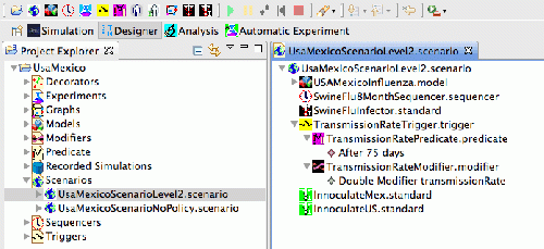
The downloadable project contains this basic model without any expressed policies. The project also contains a second scenario that shows how to set up Modifiers, Predicates, and Triggers. In this case the Modifier changes the transmission rate based on a time trigger.

Global Geographic Models Only

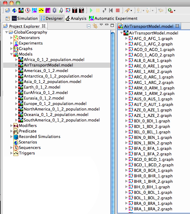
The Global Geographic Models project contains no runnable scenarios. Rather, is contains a set of pre-composed models for large regions of the world intended to be built upon in developing your own scenarios. These models, shown int he figure below, include a model for global air transportation, and a set of continent and super-continent models for geographic regions and people. After you download them, please expand them to see the inner components.

Super-Continent Examples

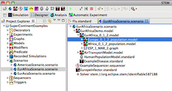
The Super-Continent Scenarios provide an examples of how to construct scenarios using the Global Model examples described above. These scenarios show how to model large regions such as the Americas, Europe+Africa, and Europe+Asia. The figure below expands the Eur-Africa Scenario. Note that the Inner Eur-Africa Model contains a model for Europe, a model for Africa, together with the connection between Spain and Morocco.