STEM Solvers

When you create a new scenario in STEM, you need to specify which solver to use. A solver is simply the method used to determine how the state of a simulation changes from one time step to the next. Models for populations and diseases in STEM are all designed to carry out this change or derivative calculation given a current state. How the derivative is applied to determine the next state is where solvers differ.

Available solvers

STEM Native Solvers

Finite Difference

The finite difference solver is the most straightforward (and fastest) solver available. It's using Euler's method and simply estimates the next value from the current value plus the derivative:

y(t+h) = y(t) +h*y'(t)

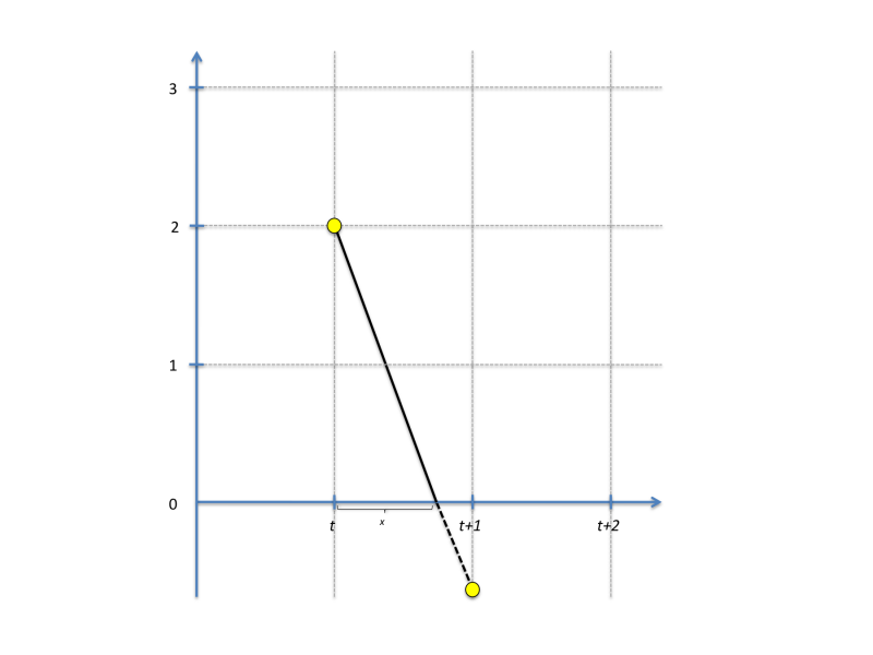
where h is the step size (default 1 day in STEM as defined by the sequencer). Label values in STEM are often constrained to a positive value. For instance, the count of a population can never go negative, and this is also true for any population assigned to a particular compartment state. When a constrained value goes negative, the finite difference solvers does a partial step to avoid this as illustrated in this figure:

(the figure assumes h = 1). The next value is thus calculated as:

y(t+h) = y(t) + x*y'(t)+(1-x)*y'(t+x)

The algorithm finds the smallest x among all differential equations solved and rescales all label values accordingly. If necessary, multiple partial steps are carried out.

The finite difference solver is able to take advance of multi-core CPUs; each CPU is assigned a sub-set of the graph to work on.

Runge Kutta Cash-Karp

The Runge Kutta Cash-Karp solver is an adaptive step size ordinary differential equation integrator that calculates six function evaluations for each time step and estimates two solutions (of 4th and 5th order). The difference between the two solutions is the estimated error, and the solver can be calibrated to any desired degree of accuracy. If the error exceeds the tolerance the step size is reduced. The Runge Kutta Cash-Karp solver can take advantage of multi-core CPUs, and each CPU is assigned a sub-set of the graphs to work on. The algorithm perform "fine-grained" CPUs synchronization to establish the step size to use, ensuring that the same solution is reached no matter how many CPUs are running concurrently or whichever way the graph is split up among the CPU cores.

Apache Commons Math solver

These solvers are using the Apache Commons Math library and its classes for solving ordinary differential equations (http://commons.apache.org/math/, http://commons.apache.org/math/userguide/ode.html).

Dormand Prince 853

The Dormand Prince 853 solver also belongs to the Runge Kutta family of ordinary differential equation integrator and adapts the step size to ensure the error is kept within acceptable bounds. The solver is using the Apache commons math library (http://commons.apache.org/math/) and the DormandPrince853Integrator class (http://commons.apache.org/math/apidocs/org/apache/commons/math/ode/nonstiff/DormandPrince853Integrator.html). Since the 1.4.1 release, this solver is able to take advantage of multi-core CPUs to increase performance.