Henshin/Conflict and Dependency Analysis

Fig. 1: Execute MultiCDA on the Henshin file or on the associated diagram file

Fig. 2: First page of the MultiCDA wizard: selecting the rules to be analysed.

Henshin's conflict and dependency analysis feature enables the detection of potential conflicts and dependencies of a set of rules. The feature is called MultiCDA in short, since it supports multiple granularity levels, which can be selected by the user.

For conflicts, there are four types of granularity:

• Binary granularity lists all conflicting rule pairs, that is, all pairs of rules from whose application a conflict can arise.
• Coarse granularity shows for each conflicting pair of rules all minimal conflict reasons. A minimal conflict reason is a minimal model fragment whose presence leads to a conflict.
• Fine granularity shows for each conflicting pair of rules all conflict reasons. A conflict reason is a model fragment whose presence leads to a conflict. General conflict reasons are obtained by different combinations of minimal ones.
• Very Fine granularity is equivalent to critical pairs, as obtained from Critical Pair Analysis (CPA). A critical pair describes a minimal conflict situation, consisting of the first rule and the second rule as well as a minimal model affected by the conflict.

For dependencies, we have the same four types of granularity, with equivalent concepts to those mentioned above: rules with a dependency, minimal dependency reasons, dependency reasons, and critical pairs. Fine and Very Fine granularity are almost identical, except for certain variations between critical pairs that are not important for most applications (explained below).

Binary-, Coarse-, and Fine-granular results are computed based on a new suite of algorithms, which are much faster than the existing CPA implementation (see Lambers et al. - Multi-granular conflict and dependency analysis in software engineering based on graph transformation). For Very Fine granularity, MultiCDA under the hood uses the existing CPA implementation.

Starting the analysis via wizard

You can execute the MultiCDA from both .henshin and .henshin_diagram files by right-clicking on it and clicking Conflict and dependency analysis beneath Henshin option, as shown in Fig. 1.

In the first page of the wizard, shows in Fig. 2, you can select first and second rules that should be analysed. There is a option to select the same rules for the right side as selected on the left side. If the Henshin file has only one rule, it is automatically selected for both sides. You can move to the next step if you choose at least one rule on each side and at least one of the kinds of the analysis: conflict and dependency. Each rule from the left side will be analysed with each rule from the right side.

Fig. 3: Second page of the MultiCDA wizard: choosing a granularity

Fig. 7: Execution of the MultiCDA analysis

In the next step the desired granularity level has to be set. In Fig. 3 you can see several options to do that, for an example rule set illustrated further in Fig. 4.

In the right pane, for the first three granularity levels, you can choose to export the results in an HTML table. There is normal and abstract way of presenting the results. The normal table is shown in the Fig. 5. On the left there are the rules that run first and above the ones that run second. In addition to the conflict types, the number of conflicts is displayed. The abstract table (Fig. 6) is showing the results between the types of rules. A kind is set with respect to the actions that exist in a rule. Each action is assigned an ID, which is explained in the legend below the table. For example, Rule d3 (Fig. 4) assigns PD as it consists of both preserve and delete elements. The abstract table is well suited for the rough overview because the rules are strongly summarized and there are no empty rows or columns. The number on the right side of each conflict kind indicates the number of existing conflicts. Reason kinds without number mean, that only one conflict of this kind was created by the given pair of rules.

• 

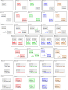
  Fig. 4: Example rule set

• 

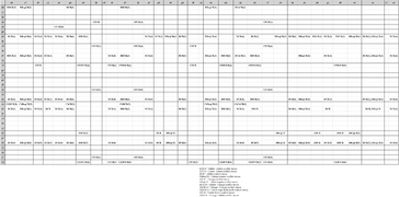
  Fig. 5: Full table for all rules from example rule set

• 

  Fig. 6: Abstract table for all rules from example rule set

The Very Fine granularity level takes three options for fine-tuning for the level of detail further (for a detailed discussion, see the opening chapters of Lambers et al., Initial Conflicts and Dependencies: Critical Pairs Revisited): Initial critical pairs returns the same amount of conflicts as the fine granularity. Compute further essential critical pairs includes as additional results a particular type of critical pair which contains isolated boundary nodes. Compute further critical pairs calculates all possible combinations of mappings of the graph elements that lead to a conflict or dependency (which may just differ in the overlapping of rule elements that are not involved in a conflict/dependency).

Once the analysis is started, the process can be cancelled at any time by clicking the red rectangle on the right side of the progress bar presented in Fig. 7. After an abort has been made, it can only be executed after the processing of the current rule pair. To provide the abort functionality, the rule pairs had to be passed to the CPA and MultiCDA individually and not at ones as in the past. This leads to a performance penalty for computing Very Fine granularity results, but not for the other granularity levels. Since the CPA has previously worked with bad runtimes, it was decided to accept the deterioration of the runtime to support the abort function.

The dialog shows the remaining time, the percentage of progress, the rule pair currently being analyzed, and the type of analysis being performed.

Inspecting results

• 

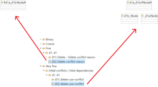
  Fig. 8: Representation of the result, showing a a delete-delete conflict reason to the left and the corresponding critical pair to the right

• 

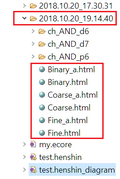
  Fig. 9: Storage of results and tables

• 

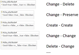
  Fig. 10: Representation of conflicts on attributes

After calculation is completed, the results are listed in the CDA\ Results window. The upper level is the granularity kind. These contain the rule pairs that are in conflict to each other. With the granularity Very fine, there is a further division into the three analysis types before the rule pairs are displayed. Each rule pair contains a set of conflicts that can be viewed by double-clicking. Fig. 8 illustrates two equal conflicts, one calculated with Fine and the other with Very Fine granularity. It is easy to see that the result for Fine is clearer, since only the conflict elements are shown there, whereas Very Fine results represent the minimum graph necessary for the execution of both rules. For this reason, the result can be confusing with complicated rules.

Fig. 9 shows how the data in the project tree view is stored. In the folder containing the Henshin file that was used for the analysis, the result folder will be created. The new folders name is the date and time the analysis took place. Unlike the CDA\ Results view, this folder contains all the Reasons and atoms together in a rule pair folder. The html tables are saved in the new folder and can be simply clicked on. The a behind the granularity name means it is an abstract representation of the results.

Fig. 10 shows the representation of the conflicting attributes. Since an attribute has the property to change the value, it was decided to show both the value of LHS and RHS. The change is represented by an arrow ->. For example, the representation true->false means that the value has changed from true to false. The value of the attribute from the first rule is separated from the second rule by an underscore, just as in the case of nodes. The x represents the nonexistent value of attribute.