Notice: this Wiki will be going read only early in 2024 and edits will no longer be possible. Please see: https://gitlab.eclipse.org/eclipsefdn/helpdesk/-/wikis/Wiki-shutdown-plan for the plan.
Henshin/State Space Tools
To verify the correctness of transformations, Henshin provides tools for generating and analyzing the state spaces of in-place model transformation. Starting from some initial state, the transformation is executed in a stepwise fashion and can be, thus, analyzed, e.g. to make sure that all intermediate states are correct fulfill some invariants.
The state space tools in Henshin currently support the following features:
- Efficient (multi-threaded), resumable generation of explicit state spaces
- State-based abstractions:
- Ignoring link orders (graph isomorphy)
- Ignoring certain attributes
- Optional object IDs
- Interactive state space generation and visualization
- Extensible validation/verification framework:
- Extensible export functionality:
- TikZ (*.tex)
- CADP (*.aut)
- PRISM (*.sm, *.nm, *.tra etc.)
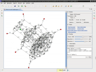
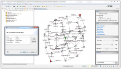
All these functionalities are integrated in a graphical state space explorer, shown on the right. They can be also invoked from the context menu for state space files or programmatically. For model checking, the state space explorer provides a uniform front-end to the above mentioned analysis tools.
State space generation
In this section, we explain how to generate a state space for a Henshin transformation.
Transformation rules and initial state
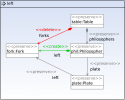
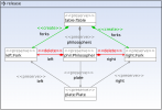
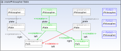
As a running example we consider the academic example of dining philosophers. To make it more interesting we include a rule for a dynamic reconfiguration, i.e. to allow to add a philosopher to the table during the execution. The rules can be specified using the either the graphical or tree-based transformation editor. The graphical versions of our rules are depicted below. We have the following rules:
- left and right for picking up forks (right is symmetric to left )
- release for putting them back on the table
- create for adding a new philosopher to the table.
Adding philosophers without an upper limit would result in an infinite state space. Therefore, we include negative application conditions (NACs) in the rule create to make sure that we cannot add arbitrarily many philosophers. Here we chose an upper limit of at most 5 philosophers.
To generate a state space, we need to specify an initial configuration. We use dynamic EMF here, that means we do not generate model classes for the EMF model. Therefore, we need to use a dynamic instance model for the initial state. To create such a dynamic instance, right-click on an *.ecore file in the package explorer and select Henshin -> Create Dynamic Instance. Now open the generated *.xmi file in the Sample reflective editor of EMF and specify the initial configuration.
Setting up the state space
Now we set up our state space file. Open the New... wizard and select Henshin State space in the Henshin category. After finishing the wizard a new file with the extension statespace is created and opened in the graphical state space explorer.
On the right-hand side you can find control panel for the explorer. On the top, the number of states, transitions and rules is displayed. Now, from the Tasks menu in the control panel, you need to do the following things:
- Import transformation rules to be used in the state space generation.
- Load one or more initial state models into the state space.
In our dining philosophers example, we import the rules left, right, release and create. As initial state, we load the file from above.
Building up the state space
The initial state appears as a green node in the state space explorer. You can click on Start layouter in the Tasks menu on the right-hand side of the explorer to enable automatic layouting. By double clicking on a state, you can unfold this state and thereby, manually explore the state space. States are depicted using different colors:
- Green: initial states
- Grey: explored states
- Blue: open states (can be explored by double clicking on them)
- Red: deadlock or terminal states (no rules are applicable here)
You can also let the tool do the work for you by clicking on Start explorer to automatically build up the state space. This can be combined with the automatic layouter.
After a number of steps, the state space for the philosophers example is fully generated. It should look more or less like in the screenshot on the right. Here we used graph equality without extra options.
Offline state space generation
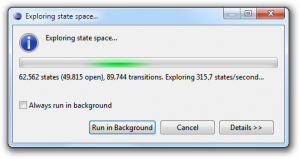
State space can be also generated outside of the graphical explorer, which is, of course, much more efficient. The offline state space generation can be invoked by clicking on Explore State Space in the State Space submenu in the context menu of state space files. On multi-core machines, a multi-threade state space exploration scheme is used, which can increase the performance by a factor, depending on the number of cores and the available memory. Note that the speed is a tradeoff between memory consumption and used time. You can also generate the state space programatically:
// Loading:
StateSpaceResourceSet resourceSet = new StateSpaceResourceSet("my/working/directory");
StateSpace stateSpace = resourceSet.getStateSpace("myexample.statespace");
StateSpaceManager manager = StateSpaceFactory.eINSTANCE.createStateSpaceManager(stateSpace, 4);

// Exploring:
StateSpaceExplorationHelper helper = new StateSpaceExplorationHelper(manager);
helper.doExploration(-1, new NullProgressMonitor());
You can also click on Properties in the context menu of state space files to see its details, e.g. the number of states. Note that statespace files have a binary format and can get large, depending on the size of the state space. The generator is currently able to handle state spaces with millions of states and tens of millions of transitions. You can open such big files also in the graphical explorer, but they will not be visualized anymore.
Resetting the state space
Another often used functionality is to reset a state space. This removes all derived state space (all states which are not initial). You can do this also from the context menu of state space files, or in the Tasks menu in the graphical explorer. You can also reset a state space programmatically:
manager.resetStateSpace();
Setting properties
You can influence the state space generation using properties associated to the state space. You can use an action in the control panel to change the options. Some common properties are the following: checkLinkOrder determines whether graph isomorphy of Ecore equality should be used (default is false). identityTypes is a comma-separated list of class names for which unique object IDs will be generated (required for parameterized actions). ignoredAttributes is a comma-separated list of attribute names whose values will be ignored when comparing states.
Setting rule priorities
By default, in every state the explorer tries to apply all imported rules. This an be further customized by assigning priorities to the rules. This is done using properties as explained in the previous paragraphs. All rules have per default the priority 0. If you have a rule called myCoolRule you can change its priority by setting the property priorityMyCoolRule to an integer value (can be also negative). Higher values mean higher priority. The semantics is as follows: in every state the explorer tries first to apply all rules with the highest priority. If at least one rule is applicable, then the rules with lower priorities are not applied. If none of the rules was applicable, then the rules with the next lower priority are tried to be applied, and so forth. This is essentially the approach of layered graph grammars. Note that priorities are only supported in Henshin 0.9.7 or higher.
Parameterized actions
In the basic version, transitions are labeled just with rule names, e.g. left and right in our simple example. A more powerful approach is also supported, which allow to parameterize the transition labels with identifiers of nodes.
To use parameters in the state space tools, add parameters to the rules you are using and use the parameter names as names for nodes in the rules. Then, make sure that the property identityTypes contains all types which are used as parameters of rules (see above). When you now regenerate the state space, you will see the parameters on the transition labels. These parameterized actions can be also very useful for model checking later (see the paragraph on model checking with parametrized actions).
State space analysis
To analyze a generated state space, open it in the graphical explorer and make sure it is fully explored (it has no open states). Then you can use the Validation menu in the control panel to analyze it.
Structural invariants in OCL
You can specify OCL constraints in the validation tool in the explorer and check them for your state space. For example in the dining philosophers state space we can check the following constraint:
self.forks->size() > 0
meaning that there is always at least one fork on the table. After having selected OCL (invariant) in the drop down menu, we can simply click on Run to check the constraint. In out case this should give us a negative result. Moreover, a trace into a state which does not fullfil the constraint is automatically selected in the explorer. This gives you essentially a counterexample for your invariant.
Qualitative model checking with CADP and mCRL2
Full model checking of temporal properties is supported using external model checkers. For qualitative model checking you can currently use either CADP or mCRL2. To use the tools in Henshin you have to install it somewhere on your computer. Note that CADP requires an (academic) license, whereas mCRL2 is open source.
When you have installed either of the tools, make sure they are in the system-wide PATH, so that Henshin can find them. For CADP you also have to define the environment variable CADP, which should point to the directory where it is installed.
Now you can model check your state space. Both mCRL2 and CADP support the modal mu-calculus which has a great raw expressive power, but is also hard to read/write. As an example, freedom of deadlock can be verified using the formula:
[true*]<true>true
In our example, this should evaluate to false. CADP moreover generates a counterexample, which is shown in the explorer (here it is a trace into one of the deadlock states). Another property that we can check is the following:
<true*>nu X.<left.right>X
which basically says: Is there an infinite sequence of the actions left and right? This should evaluate to false. However, if we try:
<true*>nu X.<left.right.release>X
we get true. Note that in CADP you have to put quotes around the action names.
Model checking with parametrized actions
State space with parameterized actions can be also analyzed. Currently, mCRL2 can be used for this. The type of the actions is induced by the parameter definitions for rules. In the following, we use the example with parameterized actions from above. We can use the parameterized actions in the model checking. For instance, consider the following formula:
[true*](forall f1,f2:Fork . exists p:Philosopher .
(
    [left(p,f1).right(p,f2)] (nu X. mu Y. ([release(p,f1,f2)]X && [!release(p,f1,f2)]Y)))
)
It states: for all forks f1,f2 there exists a philosopher, such that first left(p,f1) followed by right(p,f2) and then eventually release(p,f1,f2). This property is satisfied in our example.
For more information on the specification language check out the mCRL2 manual or the CADP manual.
See also this article on this topic. Note that the mCRL2-based approach currently does not scale very well and is limited to examples with not more than a couple of thousands of states.
Stochastic and probabilistic model checking with PRISM
Henshin supports the analysis of stochastic and probabilistic graph transformation systems using PRISM model checker.
Stochastic graph transformation systems
Henshin support stochastic graph transformation systems (SGTSs) as introduced by Heckel et al. Based on given user-defined rates for the transformation rules, Henshin generates a so-called continuous-time Markov chain (CTMC) in the input format of PRISM.
A standard task for CTMCs is to compute so-called steady-state probabilities for a state space. In essence, this analysis yields probabilities for your system being in a certain state.
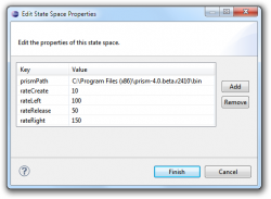
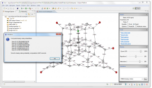
To compute steady-state probabilities in the Henshin explorer choose the tool PRISM CTMC (steady-states). Before running this tool, you should specify application rates for all rules first. This can be done by editing the properties of the state space. For a rule called myRule, its rate is specified using the property with the key rateMyRule. Rates must be specified as integers or doubles. You can also define a rate based on another rate, e.g. rateRuleA = 1-rateRuleB. The screenshot on the left shows some example rates. Note that you can also specify optional parameters for PRISM using the prismParams properties. Make sure that the prism executable is in your path. Now you can generate the steady-state probabilities, as shown in the screenshot on the right.
Using PRISM, we can check CSL properties for state spaces generated by Henshin. You need to identify a set of target states for which you want to compute the probability for. We recommend to check out the very nice documentation in the PRISM manual on property specification for this. However, a standard state property supported by PRISM is "deadlock". You can compute the probability for eventually reaching a deadlock with the following formula (this will actually produce either 0 or 1):
P=? [ F "deadlock" ]
To compute the probability for ending up in some specific states, e.g. in state 13 or 17, you can use this:
label "target" = s=13 | s=17;
P=? [ F "target" ]
You can also use OCL to specify the target states, e.g.:
label "target" = <<<OCL
   self.philosophers->size() > 4 and
   self.philosophers->size() = self.forks->size()
>>>
P=? [ F "target" ]
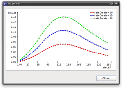
PRISM supports a so-called experiments which are essentially a sequence of model checking runs in which one parameter is changed. Based on this approach it is possible to generate plots that show how a numerical property changes if another one is changed. This feature is also supported by the PRISM adapter in Henshin's state space tools.
The only thing that you have to do is to replace some of the concrete rates for the rules by intervals. For instance, specifying the property rateLeft as 10:10:250 means that PRISM will compute the result for values 10, 20, 30, ..., 250 for rateLeft. You can do this with multiple parameters. In that case, you should specify which parameter is used for the X-axis. For instance, to vary the parameter rateLeft you need to set the following state space property: prismExperiment=rateLeft.
The Henshin tool will invoke PRISM with the correct parameters, parse the output and generate a plot such as the one in the screenshot on the right.
Probabilistic graph transformation systems
Probabilistic graph transformation systems (PGTSs) are another quantitative model. The formal details are described in an article accepted for ICGT 2012.
The usage principles of the tool for probabilistic transformation systems are the same as for stochastic transformation systems (see above). The only difference is how probabilistic rules and probabilities are specified.
In probabilistic graph transformation systems, rules have multiple right-hand sides, each of them annotated with a probability. In Henshin, you need to specify multiple rules with the same LHS (and nested conditions) and the same name. To specify probabilities for the different rules (RHSs), you can use the properties probXXX1, probXXX2, ... where XXX is the rule name with capitalized first letter (cf. the specification of rates in the stochastic case above). This is all information you need to specify. The state space tool will automatically generate a PRISM specification according to the semantics of probabilistic graph transformation systems. See also the probabilistic broadcast.
State space export
Several export formats are supported. To export a state space, either right-click on the state space file in the package explorer and choose State Space -> Export State Space or invoke use the task Export state space in the state space explorer.
CADP (*.aut)
Produces an LTS in the Aldebaran format. No parameters are required for this format.
PRISM CTMC (*.sm, *.tra)
Produces a continuous-time Markov chain (CTMC) in the input format of PRISM according to the semantics of stochastic graph transformation systems. If you choose an *.sm file, the model will be exported into the PRISM specification language. If you choose a *.tra file, the model will be exported as a transition matrix, which can be more efficiently parsed by PRISM.
As parameters, you can specify target states using OCL invariants, e.g.:
label "T1" = <<<OCL self.philosophers->size() < 2 >>>
label "T2" = <<<OCL self.philosophers->size() > 3 >>>
PRISM MDP (*.nm, *.tra)
Produces a Markov decision process (MDP) in the input format of PRISM according to the semantics of probabilistic graph transformation systems. If you choose an *.nm file, the model will be exported into the PRISM specification language. If you choose a *.tra file, the model will be exported as a transition matrix, which can be more efficiently parsed by PRISM.
You can use parameters as for CTMCs to specify target states.
TiKZ (*.tex)
Produces a graphical representation of the state space for LaTeX.

